Absence of evidence, a composite that could not succeed, and the outcome that matters
A critical re-analysis of the CMR GUIDE trial (JAMA 2026): the composite endpoint, compatibility curves and S values, a Bayesian reading, and simulations of what the trial could detect
The CMR GUIDE trial, published in JAMA in August 2026, randomized patients with a left ventricular ejection fraction of 36% to 50% and myocardial scar on cardiac MRI to a primary prevention ICD or an implantable loop recorder. Its conclusion was blunt: the ICD “did not reduce” the composite of sudden cardiac death or hemodynamically significant ventricular arrhythmia. I think that conclusion is wrong, and wrong in an instructive way. It combines a clinical problem, a composite outcome that an ICD could hardly improve, with a statistical one, absence of evidence reported as evidence of absence. Below I work through both, with all the R code, using the same tools I teach in my graduate course on evidence synthesis.
CMR GUIDE randomized 353 patients with LVEF 36% to 50% and CMR-defined scar to a primary prevention ICD (n = 180) or an implantable loop recorder (ILR, n = 173), and followed them for a median of 6.3 years (Selvanayagam et al., JAMA 2026). The abstract concludes that “implantation of an ICD did not reduce the composite outcome of SCD or HSVA”.
res<-filter(res, !is.na(hr))# analyses below use the outcomes with a reported HR
Non-cardiovascular deaths (12 vs 6) appear only in the supplement (eTables 1 and 2); the paper reports no HR for them and does not discuss the imbalance. Its Discussion refers instead to “the low competing nonarrhythmic mortality”.
Two numbers frame everything that follows. The primary result, HR 0.76 (95% CI 0.37 to 1.58), is compatible with anything from a 63% reduction to a 58% increase. And the trial planned 51 primary events but observed 30.
2 The clinical question: is “SCD or HSVA” a sensible endpoint?
2.1 The components are not of equal value
A composite assumes its components matter roughly equally to patients and respond similarly to treatment. Neither holds here. A patient would far rather survive a ventricular arrhythmia with syncope than die of it, and the two components moved in opposite directions: SCD HR 0.26, HSVA HR 1.77.
2.2 The ICD turns one component into the other
An ICD does not prevent ventricular arrhythmias; it terminates them. The arrhythmia that would have killed a patient in the ILR arm is shocked in the ICD arm, and if it caused syncope or hypotension before the shock, it is counted as HSVA. The device therefore moves events from the SCD column into the HSVA column, and the composite counts them either way. The authors say as much in their Discussion (“the most plausible explanation is that ICD therapy reduced SCD by terminating fatal ventricular arrhythmia … leading to a numerically greater number of nonfatal HSVA events”).
The DAG makes the problem explicit. Serious ventricular arrhythmias lie on the causal pathway in both arms, and randomization does not change how often they occur. What the ICD changes is the next node, whether the arrhythmia is fatal. Both branches, fatal (SCD) and survived (HSVA), feed the trial’s primary outcome, so the device’s effect cancels inside the composite. Each arm also has paths to cardiovascular death that bypass shockable arrhythmias (heart failure, bradyarrhythmias), and possibly paths to total mortality that bypass the heart altogether (device infection, sepsis, other non-cardiovascular deaths), which is where the 12 vs 6 non-cardiovascular deaths sit.
Dark boxes: the outcomes that matter to patients. Dashed grey boxes: the trial’s primary outcome and its nonfatal component.
If the ICD works only through this mechanism, the true HR for the composite is 1 however well the device works. The observed counts fit that pattern closely:
(In the ICD arm 3 + 12 = 15 events but 14 patients with a primary event: one patient had HSVA and later died suddenly. The composite counts only the first event.)
Serious arrhythmias occurred about equally often (15 vs 16), but 62% were fatal without an ICD and 20% with one. The ILR arm adds a second route: 6 ILR patients received a secondary prevention ICD after a primary outcome event, which protects them from later SCD and dilutes the SCD comparison.
The primary endpoint was therefore close to guaranteed to be null whatever the ICD did. It answers “does an ICD reduce the occurrence of serious ventricular arrhythmias?”, to which the expected answer is no. It does not answer “does an ICD prevent death?” (simulated in Section 4).
2.3 Which deaths were sudden?
Sudden, cardiovascular and total mortality blur into each other, and in an open-label device trial the classification of a death matters a great deal. The supplement (eTable 2) lists every death:
Seven fewer sudden deaths with an ICD were offset by six more non-cardiovascular deaths, leaving all-cause mortality unchanged (20 vs 19). Whether this is chance, the competing risk of older patients saved from SCD dying of something else, or misclassification cannot be settled with 39 deaths. All-cause mortality, the one outcome immune to classification, is the most patient-relevant and the least informative here: HR 0.91 (0.49 to 1.71). The data cannot exclude a 51% reduction in mortality, nor a 71% increase, although harm of that size seems unlikely. That is the key message: the question is still open, and more research is needed. How much more is sobering: detecting a 20% reduction in all-cause mortality with 80% power needs about 630 deaths (Schoenfeld); this trial had 39.
2.4 Accounting for patients (Figure 1)
Figure 1 is a CONSORT diagram, not a subtraction: it lists what happened to patients after randomization (deaths, discontinuations, losses), then returns to all 180 and 173 because the primary analysis is by intention to treat. The boxes can be checked against eTable 1:
The ICD column only adds up if all 20 deaths occurred among the 159 implanted patients, but footnote b says 2 of them never received an ICD (which would give 133). For the ILR, Figure 1 reports 8 lost to follow-up and eTable 1 reports 4; only the latter reconciles with the 118. These are small bookkeeping inconsistencies that do not change the results, but they are the kind a careful reader of a CONSORT diagram should check.
3 The statistical question: does the evidence support “did not reduce”?
3.1 Absence of evidence: the compatibility curve
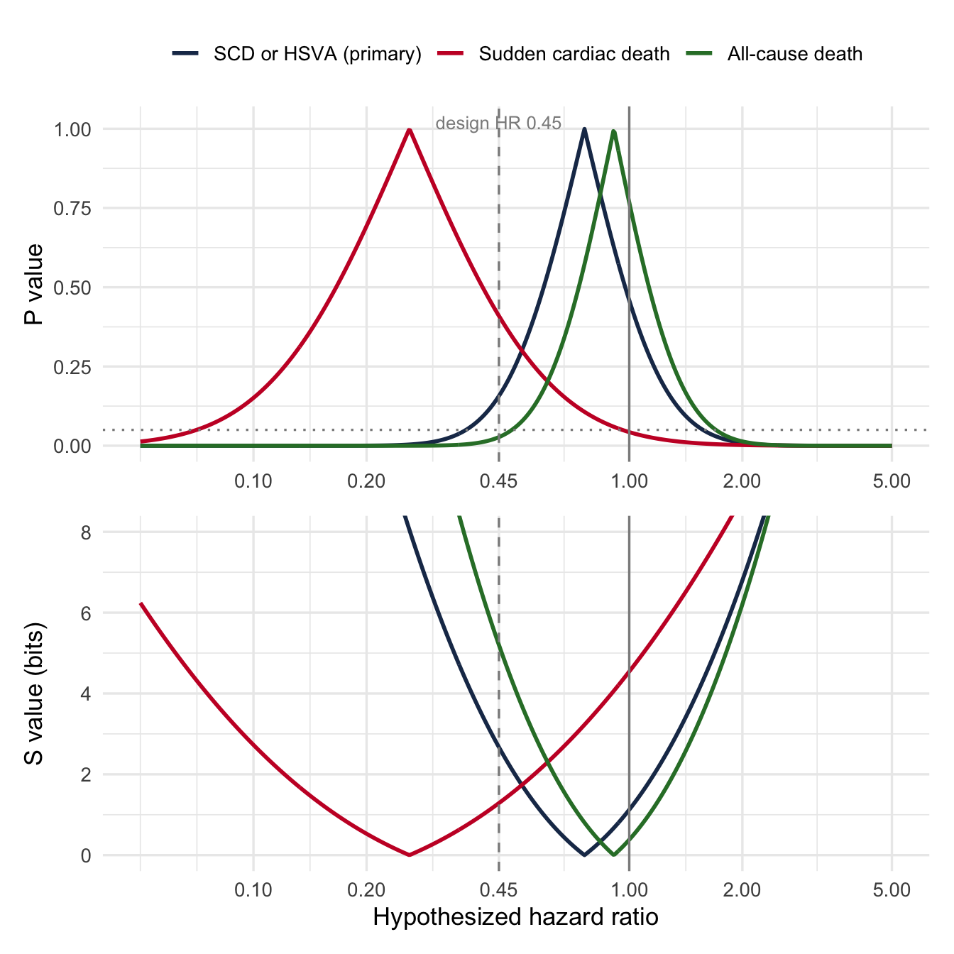
A P value of 0.46 tests one hypothesis, HR = 1. The P value function (compatibility curve) tests them all, and the S value, −log₂(P), expresses each as bits of surprise (Greenland 2019; lecture 11).
sv<-function(i, h0){p<-2*pnorm(-abs((res$loghr[i]-log(h0))/res$se[i])); c(p =p, s =-log2(p))}s_null<-sv(1, 1); s_des<-sv(1, 0.45)
For the primary outcome, the data carry 1.12 bits of information against “no effect” (P = 0.46) and 2.67 bits against the investigators’ own design hypothesis of HR 0.45 (P = 0.16). One bit is the surprise of a single fair coin landing heads; two to three bits, of two or three heads in a row. The trial barely discriminates between “no effect” and “a 55% reduction”, so it cannot support the conclusion that the ICD “did not reduce” the outcome (Altman & Bland 1995).
3.2 Surprisal, information and entropy
The S value is Shannon’s surprisal, or self-information: an event of probability p carries −log₂ p bits of information. Applied to a P value, it measures how much information the data supply against the tested hypothesis, on an additive scale: 4.3 bits (P = 0.05) is like four or five heads in a row from a coin we are testing for fairness.
Entropy is expected surprisal, H = E[−log₂ p]. When the tested hypothesis is true, a valid P value is uniformly distributed, so its surprisal has an exponential distribution with mean 1/ln 2 ≈ 1.44 bits: the average information against a true null. In other words, if “no effect” were true and the trial were repeated many times, the typical result would carry about 1.4 bits against “no effect” purely by chance. CMR GUIDE’s P value of 0.46 corresponds to 1.12 bits, about the surprise of one coin landing heads, and less than a true null would produce on average. Far from showing that the ICD has no effect, the result would be unremarkable whether the ICD had no effect or a substantial one (next table).
The surprisal curve also lets us compare hypotheses, as long as we remember that each S value is a test of one hypothesis, not a comparison of two:
Code
loghr<-res$loghr[1]; se<-res$se[1]s_of<-function(h)-log2(2*pnorm(-abs((loghr-log(h))/se)))half_s<-exp(loghr-se*qnorm(1-2^(-s_of(1)/2)/2))# benefit-side HR with half the null's surprisalhyp<-tibble(hr0 =c(1, exp(loghr), half_s, 0.45), Hypothesis =c("No effect (HR 1)", "Point estimate", "Half the surprisal of the null", "Design hypothesis"))|>mutate(P =2*pnorm(-abs((loghr-log(hr0))/se)), `S value (bits)` =-log2(P), `log2 LR vs null (bits)` =(((loghr-0)/se)^2-((loghr-log(hr0))/se)^2)/(2*log(2)))hyp|>transmute(Hypothesis, `HR tested` =f2(hr0), P =f2(P), `S value (bits)` =f2(abs(`S value (bits)`)), `log2 LR vs null (bits)` =f2(`log2 LR vs null (bits)`))|>kable()
Hypothesis
HR tested
P
S value (bits)
log2 LR vs null (bits)
No effect (HR 1)
1.00
0.46
1.12
0.00
Point estimate
0.76
1.00
0.00
0.40
Half the surprisal of the null
0.65
0.68
0.56
0.27
Design hypothesis
0.45
0.16
2.67
-1.05
The data are twice as surprising under “no effect” as under a 35% reduction (HR 0.65), yet the trial is reported as showing that the ICD “did not reduce” the outcome. Nothing in the data favours the null over a substantial benefit; the conventional reading simply privileges the null because it was the hypothesis tested. The last column makes the comparison directly: the log likelihood ratio, in bits, of each hypothesis against the null. A positive value means the data support that hypothesis more than “no effect”: both the point estimate and a 35% reduction do. Even against the design HR of 0.45 the null is favoured by only about 1.05 bit, a likelihood ratio of about 2.07, which is weak evidence by any standard.
3.3 A Bayesian reading with a vague prior
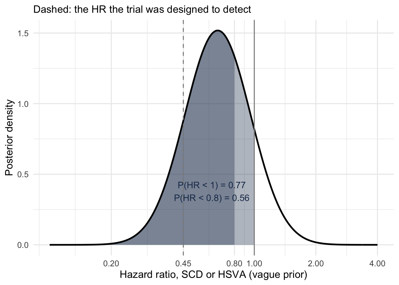
With a vague prior, normal on the log HR with SD 10, the posterior is essentially the likelihood: log HR ~ N(estimate, SE²). A skeptical prior centred on no effect, with 95% of its mass between HR 0.5 and 2 (SD 0.35), shows how much the conclusions depend on prior belief (lecture 13).
With a vague prior, the probability that the ICD reduced the primary outcome is 0.77, and the probability of a reduction of 20% or more is 0.55. That is uncertainty, not evidence of no effect. Equally, the probability that the ICD increased the primary outcome is 0.23: even the direction of the effect, its sign, is uncertain. For sudden cardiac death the probability of benefit is 0.98 with a vague prior and 0.83 even with a skeptical one.
3.4 Power: the trial was designed on projections that proved wrong
Power is a property of a design: it is computed before the trial, from projected event rates and an assumed effect. Once the results are known it has no role in interpreting them. “Observed” (post hoc) power, calculated at the observed effect, is simply a re-expression of the P value and adds nothing (Hoenig & Heisey 2001); after the trial, precision is judged from the confidence interval and the compatibility curve above.
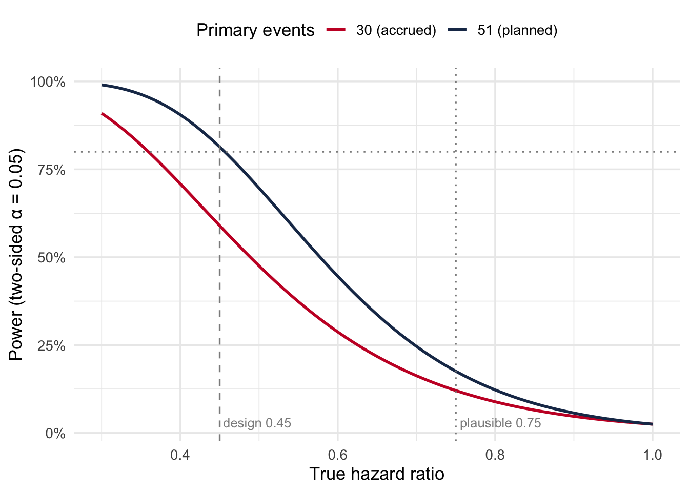
What power can show is whether the design was realistic. The trial planned 51 events, enough for 80% power to detect HR 0.45, by projecting an annual SCD rate of 4% in the control arm. The rate turned out to be 1.1%, and only 30 events accrued. The plot shows the power curves a design-stage calculation would have produced for 51 events and for 30.
Schoenfeld’s formula gives 49 events for HR 0.45, matching the protocol. Had the event rate been projected correctly, the same calculation at the design stage would have shown a trial of 30 events to have 59% power for HR 0.45 and 12% for a more plausible 25% reduction: a design no funder or ethics board should have accepted.
Was HR 0.45 a clinically relevant threshold? It reads more like the effect needed to make the trial affordable. A 55% reduction would exceed what ICDs achieved on all-cause mortality in the trials that established them (HR about 0.7 to 0.8), and the composite was diluted by HSVA, which the ICD cannot prevent and may increase. The question a clinician would ask, the smallest reduction in sudden death worth a device with a 16% rate of device-related complications and worse quality of life, was never posed.
4 Simulations: what this trial could and could not detect
Each simulated trial mimics CMR GUIDE: 180 and 173 patients, administrative follow-up of 3.5 to 9 years, a competing non-arrhythmic death rate of 1.2% per year, and a control-arm rate of serious ventricular arrhythmia that yields about 30 primary events. In the control arm 60% of arrhythmias are fatal (10 of 16 observed). Effects are estimated as subdistribution HRs with Fine-Gray models, as in the paper, with non-arrhythmic death as the competing event.
Code
# Fine-Gray subdistribution HR, as in the paper (status: 1 = event, 2 = competing death, 0 = censored)fgfit<-function(tt, st, arm){d<-data.frame(tt =tt, st =factor(st, levels =0:2), arm =arm)fg<-finegray(Surv(tt, st)~., data =d, etype ="1")m<-coxph(Surv(fgstart, fgstop, fgstatus)~arm, weights =fgwt, data =fg)unname(c(coef(m), sqrt(vcov(m))))}sim_trial<-function(hr_arr=1, rescue=0, p_fatal=0.6, lam=0.015,lam_cr=0.012, n=c(icd =180, ilr =173)){arm<-rep(c(1, 0), n); N<-length(arm)# 1 = ICDt_va<-rexp(N, lam*ifelse(arm==1, hr_arr, 1))# first serious ventricular arrhythmiat_cr<-rexp(N, lam_cr)# non-arrhythmic death (competing)cens<-runif(N, 3.5, 9)# administrative follow-upfirst<-pmin(t_va, t_cr, cens)va<-t_va==first; cr<-t_cr==firstfatal<-va&rbinom(N, 1, p_fatal*ifelse(arm==1, 1-rescue, 1))==1# composite: first arrhythmia, with non-arrhythmic death competingst_comp<-ifelse(va, 1, ifelse(cr, 2, 0))# SCD: survivors of a nonfatal arrhythmia stay at risk of a competing death until censoringt_after<-pmin(t_cr, cens)tt_scd<-ifelse(fatal, t_va, ifelse(va, t_after, first))st_scd<-ifelse(fatal, 1, ifelse(va, ifelse(t_cr<cens, 2, 0), ifelse(cr, 2, 0)))comp<-fgfit(first, st_comp, arm); scd<-fgfit(tt_scd, st_scd, arm)c(events =sum(va), hr_comp =exp(comp[1]), p_comp =2*pnorm(-abs(comp[1]/comp[2])), scd_events =sum(fatal), hr_scd =exp(scd[1]), p_scd =2*pnorm(-abs(scd[1]/scd[2])))}run<-function(label, nsim=2000, ...){args<-list(...)# replicate() cannot pass ... through directlyset.seed(629)out<-replicate(nsim, do.call(sim_trial, args))as_tibble(t(out))|>mutate(scenario =label)}
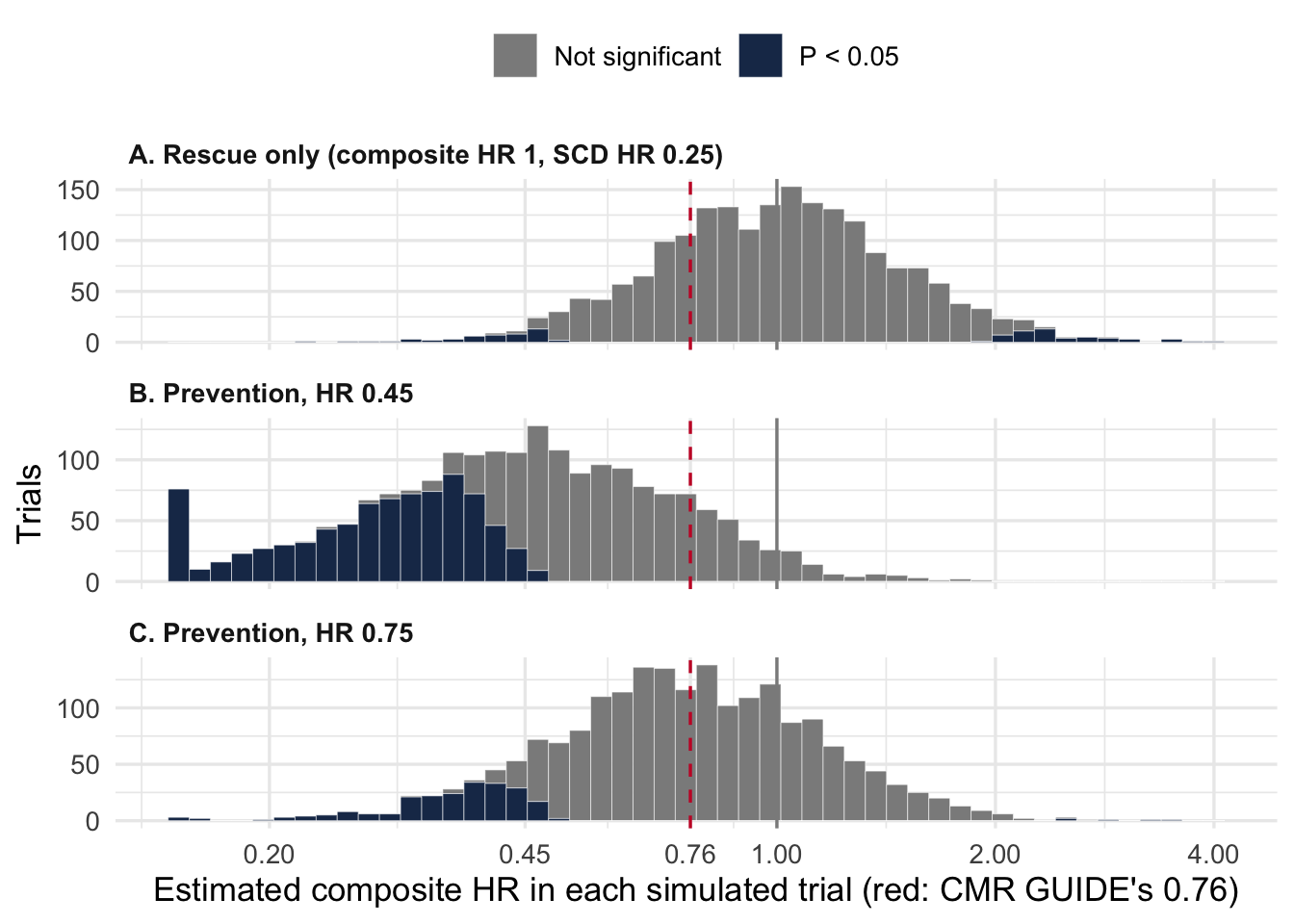
Three truths are simulated:
A. Rescue only: the ICD does not change how often serious arrhythmias occur but rescues 75% of those that would have been fatal. The true composite HR is 1; the true SCD HR is 0.25.
B. Prevention, design effect: the ICD reduces the composite by 55% (HR 0.45), the investigators’ assumption.
C. Prevention, realistic effect: the ICD reduces the composite by 25% (HR 0.75).
sims|>filter(is.finite(hr_comp), hr_comp>0)|>mutate(sig =if_else(p_comp<0.05, "P < 0.05", "Not significant"), hr_plot =pmin(pmax(hr_comp, 0.15), 4))|># pile extreme estimates at the edgesggplot(aes(hr_plot, fill =sig))+geom_histogram(bins =50, colour ="white", linewidth =0.1)+geom_vline(xintercept =1, colour =grey)+geom_vline(xintercept =0.76, linetype ="dashed", colour =red)+facet_wrap(~scenario, ncol =1, scales ="free_y")+scale_x_log10(breaks =c(0.2, 0.45, 0.76, 1, 2, 4))+scale_fill_manual(values =c(grey, navy), name =NULL)+labs(x ="Estimated composite HR in each simulated trial (red: CMR GUIDE's 0.76)", y ="Trials")+theme(legend.position ="top", strip.text =element_text(face ="bold", hjust =0))
The simulations make three points.
Under scenario A the composite cannot detect the ICD at all. Its “power” is 5%, the false-positive rate, even though the device prevents three in four sudden deaths; and even the SCD component reaches P < 0.05 in only 49% of trials. A null composite is exactly what an effective ICD would produce.
The investigators’ own hypothesis is detected in fewer than half the trials (41%, scenario B) at the event rates actually observed, and a realistic 25% reduction (C) in only 11%.
The reverse of the winner’s curse. When a true benefit is missed, the estimate is not a small, honest underestimate. Under a true 25% reduction, 23% of trials estimate HR ≥ 1, so the device looks useless or harmful in about one trial in four where it truly helps. “Not significant” in an underpowered trial says almost nothing about the size, or even the direction, of the effect.
5 The other direction: Type S and Type M errors for the “significant” findings
Low power does not only hide true effects; when a result does cross P < 0.05, it exaggerates them (Gelman & Carlin 2014). Two “significant” results in this paper qualify: the SCD component (HR 0.26) and the age < 70 subgroup (HR 0.28).
If the true effect of an ICD on sudden death is similar to DANISH (HR 0.50, eTable 4), a trial this small detects it only about one time in five, and when it does, the log HR is exaggerated about 2.4-fold on average, enough to turn a true HR of 0.5 into a reported value near 0.2 to 0.3. The age < 70 subgroup, one of six unadjusted interaction tests, is still more fragile. The SCD signal is real enough to deserve a better trial, but its size should be discounted.
6 What can be concluded
Claim
Supported?
“ICD did not reduce SCD or HSVA”
No. The data are compatible with anything from a 63% reduction to a 58% increase; P(HR < 1) = 0.77.
The composite tests the ICD’s benefit
No. An ICD converts fatal arrhythmias into nonfatal ones, so the composite is expected to be null even if the device works.
The ICD reduced sudden death
Probably (P(HR < 1) about 0.98), but the 74% reduction is likely exaggerated.
The ICD reduced all-cause mortality
Unknown: HR 0.91, compatible with a 51% reduction or a 71% increase. More research is needed.
Benefit is confined to patients under 70
Hypothesis only: one of six unadjusted subgroups, likely exaggerated.
A conclusion the data support: In patients with LVEF 36% to 50% and myocardial scar, this trial was too small, and its primary composite unsuited, to determine whether a primary prevention ICD reduces mortality. Sudden cardiac death was less frequent with an ICD, but the estimate is imprecise and probably exaggerated. The effect on all-cause mortality remains uncertain, from a large benefit to harm, and an adequately powered trial with mortality as its primary outcome is needed.
References
Selvanayagam JB, Cleland JGF, Hillis GS, et al. Cardiovascular magnetic resonance to guide defibrillator implantation for LVEF of 36% to 50%: the CMR GUIDE randomized clinical trial. JAMA. 2026;336(19):1734-1744. doi:10.1001/jama.2026.17078
Altman DG, Bland JM. Absence of evidence is not evidence of absence. BMJ. 1995;311:485. doi:10.1136/bmj.311.7003.485
Greenland S. Valid P-values behave exactly as they should: some misleading criticisms of P-values and their resolution with S-values. Am Stat. 2019;73(sup1):106-114. doi:10.1080/00031305.2018.1529625
Gelman A, Carlin J. Beyond power calculations: assessing Type S (sign) and Type M (magnitude) errors. Perspect Psychol Sci. 2014;9(6):641-651. doi:10.1177/1745691614551642
Køber L, Thune JJ, Nielsen JC, et al. Defibrillator implantation in patients with nonischemic systolic heart failure (DANISH). N Engl J Med. 2016;375:1221-1230. doi:10.1056/NEJMoa1608029
Citation
BibTeX citation:
@online{brophy2026,
author = {Brophy, Jay},
title = {CMR {GUIDE:} {Did} the {ICD} {Really} {Not} {Work?}},
date = {2026-11-20},
url = {https://brophyj.com/posts/2026-11-20-cmr-guide/},
langid = {en}
}
---title: "CMR GUIDE: Did the ICD Really Not Work?"subtitle: "Absence of evidence, a composite that could not succeed, and the outcome that matters"description: "A critical re-analysis of the CMR GUIDE trial (JAMA 2026): the composite endpoint, compatibility curves and S values, a Bayesian reading, and simulations of what the trial could detect"author: - name: Jay Brophy url: https://brophyj.github.io/ orcid: 0000-0001-8049-6875 affiliation: McGill University Dept Medicine, Epidemiology & Biostatistics affiliation-url: https://mcgill.cacategories: [Bayesian inference, RCTs, composite outcomes, absence of evidence, S values, cardiology]image: preview-image.pngcitation: url: https://brophyj.com/posts/2026-11-20-cmr-guide/date: 2026-11-20lastmod: 2026-11-20featured: truedraft: falseprojects: []format: html: theme: [simple, ../../custom.scss] code-fold: true code-tools: true embed-resources: true toc: true toc-depth: 2 number-sections: trueexecute: warning: false message: false---The CMR GUIDE trial, published in *JAMA* in August 2026, randomized patients with a left ventricular ejection fraction of 36% to 50% and myocardial scar on cardiac MRI to a primary prevention ICD or an implantable loop recorder. Its conclusion was blunt: the ICD "did not reduce" the composite of sudden cardiac death or hemodynamically significant ventricular arrhythmia. I think that conclusion is wrong, and wrong in an instructive way. It combines a clinical problem, a composite outcome that an ICD could hardly improve, with a statistical one, absence of evidence reported as evidence of absence. Below I work through both, with all the R code, using the same tools I teach in my graduate course on evidence synthesis.```{r setup}#| code-fold: truelibrary(tidyverse)library(survival)library(patchwork)library(knitr)theme_set(theme_minimal(base_size =13))navy <-"#1C3557"; red <-"#C8102E"; green <-"#2E7D32"; grey <-"grey55"f2 <-function(x) formatC(x, format ="f", digits =2)f3 <-function(x) formatC(x, format ="f", digits =3)pc <-function(x, d =0) paste0(formatC(100* x, format ="f", digits = d), "%")# log HR and its SE recovered from a reported HR and 95% CIfrom_ci <-function(hr, lo, hi) tibble(loghr =log(hr), se = (log(hi) -log(lo)) / (2*qnorm(0.975)))```# The trial in one tableCMR GUIDE randomized 353 patients with LVEF 36% to 50% and CMR-defined scar to a primary prevention ICD (n = 180) or an implantable loop recorder (ILR, n = 173), and followed them for a median of 6.3 years ([Selvanayagam et al., JAMA 2026](https://doi.org/10.1001/jama.2026.17078)). The abstract concludes that "implantation of an ICD did not reduce the composite outcome of SCD or HSVA".```{r data}res <-tribble(~outcome, ~icd, ~ilr, ~hr, ~lo, ~hi,"SCD or HSVA (primary)", 14, 16, 0.76, 0.37, 1.58,"Sudden cardiac death", 3, 10, 0.26, 0.07, 0.95,"HSVA", 12, 6, 1.77, 0.65, 4.81,"Cardiovascular death", 8, 13, 0.53, 0.22, 1.27,"Non-cardiovascular death", 12, 6, NA, NA, NA,"All-cause death", 20, 19, 0.91, 0.49, 1.71,"Heart failure hospitalization", 26, 21, 1.13, 0.63, 2.03) |>mutate(from_ci(hr, lo, hi), p =2*pnorm(-abs(loghr / se)))res |>transmute(Outcome = outcome, `ICD (n = 180)`= icd, `ILR (n = 173)`= ilr,`HR (95% CI)`=if_else(is.na(hr), "not reported", sprintf("%.2f (%.2f to %.2f)", hr, lo, hi)),`SE(log HR)`=if_else(is.na(se), "", f3(se)), P =if_else(is.na(p), "", f3(p))) |>kable()res <-filter(res, !is.na(hr)) # analyses below use the outcomes with a reported HR```Non-cardiovascular deaths (12 vs 6) appear only in the supplement (eTables 1 and 2); the paper reports no HR for them and does not discuss the imbalance. Its Discussion refers instead to "the low competing nonarrhythmic mortality".Two numbers frame everything that follows. The primary result, HR `r f2(res$hr[1])` (95% CI `r f2(res$lo[1])` to `r f2(res$hi[1])`), is compatible with anything from a 63% reduction to a 58% increase. And the trial planned 51 primary events but observed `r sum(res$icd[1], res$ilr[1])`.# The clinical question: is "SCD or HSVA" a sensible endpoint?## The components are not of equal valueA composite assumes its components matter roughly equally to patients and respond similarly to treatment. Neither holds here. A patient would far rather survive a ventricular arrhythmia with syncope than die of it, and the two components moved in opposite directions: SCD HR `r f2(res$hr[2])`, HSVA HR `r f2(res$hr[3])`.## The ICD turns one component into the otherAn ICD does not prevent ventricular arrhythmias; it terminates them. The arrhythmia that would have killed a patient in the ILR arm is shocked in the ICD arm, and if it caused syncope or hypotension before the shock, it is counted as HSVA. The device therefore moves events from the SCD column into the HSVA column, and the composite counts them either way. The authors say as much in their Discussion ("the most plausible explanation is that ICD therapy reduced SCD by terminating fatal ventricular arrhythmia … leading to a numerically greater number of nonfatal HSVA events").The DAG makes the problem explicit. Serious ventricular arrhythmias lie on the causal pathway in **both** arms, and randomization does not change how often they occur. What the ICD changes is the next node, whether the arrhythmia is fatal. Both branches, fatal (SCD) and survived (HSVA), feed the trial's primary outcome, so the device's effect cancels inside the composite. Each arm also has paths to cardiovascular death that bypass shockable arrhythmias (heart failure, bradyarrhythmias), and possibly paths to total mortality that bypass the heart altogether (device infection, sepsis, other non-cardiovascular deaths), which is where the 12 vs 6 non-cardiovascular deaths sit.```{mermaid}flowchart LR R[Randomization] --> ICD[ICD arm] R --> ILR[ILR arm] ICD -. "non-CV" .-> TM ICD -- "HF, bradyarrhythmia" --> CV ICD --> VA1[Serious VA] --> F1{Fatal?} F1 -- no --> HS1[Survived VA = HSVA] F1 -- yes --> SCD[SCD] ILR --> VA2[Serious VA] --> F2{Fatal?} F2 -- yes --> SCD F2 -- no --> HS2[Survived VA = HSVA] HS1 --> P1[[CMR GUIDE primary outcome, ICD arm]] SCD --> P1 SCD --> CV[CV mortality] SCD --> P2[[CMR GUIDE primary outcome, ILR arm]] HS2 --> P2 ILR -- "HF, bradyarrhythmia" --> CV ILR -. "non-CV" .-> TM CV --> TM[Total mortality] classDef key fill:#1C3557,stroke:#1C3557,stroke-width:3px,color:#ffffff,font-weight:bold classDef muted fill:#f7f7f7,stroke:#9e9e9e,stroke-dasharray:5 4,color:#8a8a8a class SCD,CV,TM key class HS1,HS2,P1,P2 muted```*Dark boxes: the outcomes that matter to patients. Dashed grey boxes: the trial's primary outcome and its nonfatal component.*If the ICD works only through this mechanism, the true HR for the composite is 1 *however well the device works*. The observed counts fit that pattern closely:```{r conversion}arr <-tibble(arm =c("ICD", "ILR"),scd =c(3, 10), hsva =c(12, 6)) |>mutate(arrhythmic_events = scd + hsva, fatal_fraction = scd / arrhythmic_events)arr |>mutate(fatal_fraction =pc(fatal_fraction)) |>kable(col.names =c("Arm", "SCD", "HSVA", "Serious arrhythmias", "Fatal"))```(In the ICD arm 3 + 12 = 15 events but 14 patients with a primary event: one patient had HSVA and later died suddenly. The composite counts only the first event.)Serious arrhythmias occurred about equally often (`r arr$arrhythmic_events[1]` vs `r arr$arrhythmic_events[2]`), but `r pc(arr$fatal_fraction[2])` were fatal without an ICD and `r pc(arr$fatal_fraction[1])` with one. The ILR arm adds a second route: 6 ILR patients received a secondary prevention ICD *after* a primary outcome event, which protects them from later SCD and dilutes the SCD comparison.The primary endpoint was therefore close to guaranteed to be null whatever the ICD did. It answers "does an ICD reduce the occurrence of serious ventricular arrhythmias?", to which the expected answer is no. It does not answer "does an ICD prevent death?" (simulated in @sec-sim).## Which deaths were sudden?Sudden, cardiovascular and total mortality blur into each other, and in an open-label device trial the classification of a death matters a great deal. The supplement (eTable 2) lists every death:```{r deaths}deaths <-tribble(~arm, ~SCD, ~`Other CV`, ~`Non-CV`,"ICD", 3, 5, 12,"ILR", 10, 3, 6) |>mutate(Total = SCD +`Other CV`+`Non-CV`)kable(deaths, col.names =c("Arm", "Sudden cardiac", "Other cardiovascular", "Non-cardiovascular", "All deaths"))```Seven fewer sudden deaths with an ICD were offset by six more non-cardiovascular deaths, leaving all-cause mortality unchanged (20 vs 19). Whether this is chance, the competing risk of older patients saved from SCD dying of something else, or misclassification cannot be settled with 39 deaths. All-cause mortality, the one outcome immune to classification, is the most patient-relevant and the least informative here: HR `r f2(res$hr[res$outcome == "All-cause death"])` (`r f2(res$lo[res$outcome == "All-cause death"])` to `r f2(res$hi[res$outcome == "All-cause death"])`). The data cannot exclude a 51% reduction in mortality, nor a 71% increase, although harm of that size seems unlikely. That is the key message: **the question is still open, and more research is needed.** How much more is sobering: detecting a 20% reduction in all-cause mortality with 80% power needs about `r round(4 * (qnorm(0.975) + qnorm(0.8))^2 / log(0.8)^2, -1)` deaths (Schoenfeld); this trial had 39.## Accounting for patients (Figure 1)Figure 1 is a CONSORT diagram, not a subtraction: it lists what happened to patients after randomization (deaths, discontinuations, losses), then returns to all 180 and 173 because the primary analysis is by intention to treat. The boxes can be checked against eTable 1:```{r flow}flow <-tribble(~arm, ~implanted, ~died, ~discontinued, ~lost_fig1, ~lost_etab1, ~active_end,"ICD", 159, 20, 6, 2, 2, 131,"ILR", 163, 19, 22, 8, 4, 118) |>mutate(check_fig1 = implanted - died - discontinued - lost_fig1,check_etab1 = implanted - died - discontinued - lost_etab1)kable(flow, col.names =c("Arm", "Implanted", "Died", "Discontinued", "Lost (Fig 1)", "Lost (eTable 1)","Active at end", "Implanted − exits (Fig 1)", "Implanted − exits (eTable 1)"))```The ICD column only adds up if all 20 deaths occurred among the 159 implanted patients, but footnote b says 2 of them never received an ICD (which would give 133). For the ILR, Figure 1 reports 8 lost to follow-up and eTable 1 reports 4; only the latter reconciles with the 118. These are small bookkeeping inconsistencies that do not change the results, but they are the kind a careful reader of a CONSORT diagram should check.# The statistical question: does the evidence support "did not reduce"?## Absence of evidence: the compatibility curveA *P* value of `r f2(res$p[1])` tests one hypothesis, HR = 1. The *P* value function (compatibility curve) tests them all, and the S value, −log₂(*P*), expresses each as bits of surprise ([Greenland 2019](https://doi.org/10.1080/00031305.2018.1529625); lecture 11).```{r pfun}#| fig-height: 7grid <-exp(seq(log(0.05), log(5), length.out =600))pfun <- res |>filter(outcome %in%c("SCD or HSVA (primary)", "Sudden cardiac death", "All-cause death")) |>mutate(outcome =fct_inorder(outcome)) |>reframe(hr0 = grid, p =2*pnorm(-abs((loghr -log(grid)) / se)), .by = outcome) |>mutate(s =-log2(p))p1 <-ggplot(pfun, aes(hr0, p, colour = outcome)) +geom_line(linewidth =1) +geom_vline(xintercept =c(0.45, 1), linetype =c("dashed", "solid"), colour = grey) +geom_hline(yintercept =0.05, linetype ="dotted", colour = grey) +annotate("text", x =0.45, y =1.02, label ="design HR 0.45", size =3.4, colour = grey) +scale_x_log10(breaks =c(0.1, 0.2, 0.45, 1, 2, 5)) +scale_colour_manual(values =c(navy, red, green), name =NULL) +labs(x =NULL, y ="P value") +theme(legend.position ="top")p2 <-ggplot(pfun, aes(hr0, s, colour = outcome)) +geom_line(linewidth =1) +geom_vline(xintercept =c(0.45, 1), linetype =c("dashed", "solid"), colour = grey) +scale_x_log10(breaks =c(0.1, 0.2, 0.45, 1, 2, 5)) +coord_cartesian(ylim =c(0, 8)) +scale_colour_manual(values =c(navy, red, green), guide ="none") +labs(x ="Hypothesized hazard ratio", y ="S value (bits)")p1 / p2``````{r svalues}sv <-function(i, h0) { p <-2*pnorm(-abs((res$loghr[i] -log(h0)) / res$se[i])); c(p = p, s =-log2(p)) }s_null <-sv(1, 1); s_des <-sv(1, 0.45)```For the primary outcome, the data carry `r f2(s_null["s"])` bits of information against "no effect" (*P* = `r f2(s_null["p"])`) and `r f2(s_des["s"])` bits against the investigators' own design hypothesis of HR 0.45 (*P* = `r f2(s_des["p"])`). One bit is the surprise of a single fair coin landing heads; two to three bits, of two or three heads in a row. The trial barely discriminates between "no effect" and "a 55% reduction", so it cannot support the conclusion that the ICD "did not reduce" the outcome ([Altman & Bland 1995](https://doi.org/10.1136/bmj.311.7003.485)).## Surprisal, information and entropyThe S value is Shannon's *surprisal*, or self-information: an event of probability *p* carries −log₂ *p* bits of information. Applied to a *P* value, it measures how much information the data supply against the tested hypothesis, on an additive scale: 4.3 bits (*P* = 0.05) is like four or five heads in a row from a coin we are testing for fairness.**Entropy** is expected surprisal, H = E[−log₂ *p*]. When the tested hypothesis is true, a valid *P* value is uniformly distributed, so its surprisal has an exponential distribution with mean 1/ln 2 ≈ `r f2(1 / log(2))` bits: the *average* information against a *true* null. In other words, if "no effect" were true and the trial were repeated many times, the typical result would carry about 1.4 bits against "no effect" purely by chance. CMR GUIDE's *P* value of `r f2(s_null["p"])` corresponds to `r f2(s_null["s"])` bits, about the surprise of one coin landing heads, and **less than a true null would produce on average**. Far from showing that the ICD has no effect, the result would be unremarkable whether the ICD had no effect or a substantial one (next table).The surprisal curve also lets us compare hypotheses, as long as we remember that each S value is a test of one hypothesis, not a comparison of two:```{r surprisal-table}loghr <- res$loghr[1]; se <- res$se[1]s_of <-function(h) -log2(2*pnorm(-abs((loghr -log(h)) / se)))half_s <-exp(loghr - se *qnorm(1-2^(-s_of(1) /2) /2)) # benefit-side HR with half the null's surprisalhyp <-tibble(hr0 =c(1, exp(loghr), half_s, 0.45),Hypothesis =c("No effect (HR 1)", "Point estimate", "Half the surprisal of the null", "Design hypothesis")) |>mutate(P =2*pnorm(-abs((loghr -log(hr0)) / se)),`S value (bits)`=-log2(P),`log2 LR vs null (bits)`= (((loghr -0) / se)^2- ((loghr -log(hr0)) / se)^2) / (2*log(2)))hyp |>transmute(Hypothesis, `HR tested`=f2(hr0), P =f2(P),`S value (bits)`=f2(abs(`S value (bits)`)), `log2 LR vs null (bits)`=f2(`log2 LR vs null (bits)`)) |>kable()```The data are **twice as surprising under "no effect" as under a `r pc(1 - half_s)` reduction** (HR `r f2(half_s)`), yet the trial is reported as showing that the ICD "did not reduce" the outcome. Nothing in the data favours the null over a substantial benefit; the conventional reading simply privileges the null because it was the hypothesis tested. The last column makes the comparison directly: the log likelihood ratio, in bits, of each hypothesis against the null. A positive value means the data support that hypothesis *more* than "no effect": both the point estimate and a 35% reduction do. Even against the design HR of 0.45 the null is favoured by only about `r f2(-hyp[[5]][4])` bit, a likelihood ratio of about `r f2(2^(-hyp[[5]][4]))`, which is weak evidence by any standard.## A Bayesian reading with a vague priorWith a vague prior, normal on the log HR with SD 10, the posterior is essentially the likelihood: log HR ~ N(estimate, SE²). A skeptical prior centred on no effect, with 95% of its mass between HR 0.5 and 2 (SD 0.35), shows how much the conclusions depend on prior belief (lecture 13).```{r bayes}post <-function(m, s, m0 =0, s0 =10) { w <- (1/ s0^2) / (1/ s0^2+1/ s^2)c(mean = w * m0 + (1- w) * m, sd =sqrt(1/ (1/ s0^2+1/ s^2)))}probs <-function(pm, ps) c(`P(HR < 1)`=pnorm(0, pm, ps), `P(HR < 0.8)`=pnorm(log(0.8), pm, ps),`P(HR < 0.45)`=pnorm(log(0.45), pm, ps), `P(HR > 1)`=1-pnorm(0, pm, ps))bayes_tab <- res |>filter(outcome !="HSVA") |>rowwise() |>reframe(outcome, prior =c("Vague", "Skeptical"),pm =c(post(loghr, se)["mean"], post(loghr, se, s0 =0.35)["mean"]),ps =c(post(loghr, se)["sd"], post(loghr, se, s0 =0.35)["sd"])) |>rowwise() |>mutate(as_tibble_row(probs(pm, ps)),`Posterior HR (95% CrI)`=sprintf("%.2f (%.2f to %.2f)", exp(pm), exp(pm -1.96* ps), exp(pm +1.96* ps))) |>ungroup()bayes_tab |>transmute(Outcome = outcome, Prior = prior, `Posterior HR (95% CrI)`,across(starts_with("P("), \(x) f2(x))) |>kable()``````{r bayes-plot}prim <- res[1, ]dens <-tibble(hr =exp(seq(log(0.1), log(4), length.out =800))) |>mutate(d =dnorm(log(hr), prim$loghr, prim$se) / hr) # density on the HR scaleggplot(dens, aes(hr, d)) +geom_area(data =filter(dens, hr <1), fill = navy, alpha =0.35) +geom_area(data =filter(dens, hr <0.8), fill = navy, alpha =0.35) +geom_line(linewidth =1) +geom_vline(xintercept =c(0.45, 1), linetype =c("dashed", "solid"), colour = grey) +annotate("text", x =0.62, y =max(dens$d) *0.25,label =sprintf("P(HR < 1) = %.2f\nP(HR < 0.8) = %.2f",pnorm(0, prim$loghr, prim$se), pnorm(log(0.8), prim$loghr, prim$se)),colour = navy, size =4) +scale_x_log10(breaks =c(0.2, 0.45, 0.8, 1, 2, 4)) +labs(x ="Hazard ratio, SCD or HSVA (vague prior)", y ="Posterior density",subtitle ="Dashed: the HR the trial was designed to detect")``````{r bayes-text}bp <-function(o, pr, col) bayes_tab[[col]][bayes_tab$outcome == o & bayes_tab$prior == pr]```With a vague prior, the probability that the ICD reduced the primary outcome is `r f2(bp("SCD or HSVA (primary)", "Vague", "P(HR < 1)"))`, and the probability of a reduction of 20% or more is `r f2(bp("SCD or HSVA (primary)", "Vague", "P(HR < 0.8)"))`. That is uncertainty, not evidence of no effect. Equally, the probability that the ICD *increased* the primary outcome is `r f2(bp("SCD or HSVA (primary)", "Vague", "P(HR > 1)"))`: even the direction of the effect, its sign, is uncertain. For sudden cardiac death the probability of benefit is `r f2(bp("Sudden cardiac death", "Vague", "P(HR < 1)"))` with a vague prior and `r f2(bp("Sudden cardiac death", "Skeptical", "P(HR < 1)"))` even with a skeptical one.## Power: the trial was designed on projections that proved wrongPower is a property of a *design*: it is computed before the trial, from projected event rates and an assumed effect. Once the results are known it has no role in interpreting them. "Observed" (post hoc) power, calculated at the observed effect, is simply a re-expression of the *P* value and adds nothing ([Hoenig & Heisey 2001](https://doi.org/10.1198/000313001300339897)); after the trial, precision is judged from the confidence interval and the compatibility curve above.What power *can* show is whether the design was realistic. The trial planned 51 events, enough for 80% power to detect HR 0.45, by projecting an annual SCD rate of 4% in the control arm. The rate turned out to be 1.1%, and only 30 events accrued. The plot shows the power curves a design-stage calculation would have produced for 51 events and for 30.```{r power}schoenfeld_power <-function(hr, d, alpha =0.05) pnorm(sqrt(d /4) *abs(log(hr)) -qnorm(1- alpha /2))d_needed <-4* (qnorm(0.975) +qnorm(0.8))^2/log(0.45)^2pw <-expand_grid(hr =seq(0.3, 1, by =0.01), events =c(51, 30)) |>mutate(power =schoenfeld_power(hr, events),events =factor(events, labels =c("30 (accrued)", "51 (planned)")))ggplot(pw, aes(hr, power, colour = events)) +geom_line(linewidth =1) +geom_vline(xintercept =c(0.45, 0.75), linetype =c("dashed", "dotted"), colour = grey) +geom_hline(yintercept =0.8, linetype ="dotted", colour = grey) +annotate("text", x =0.45, y =0.03, label ="design 0.45", size =3.4, colour = grey, hjust =-0.05) +annotate("text", x =0.75, y =0.03, label ="plausible 0.75", size =3.4, colour = grey, hjust =-0.05) +scale_colour_manual(values =c(red, navy), name ="Primary events") +scale_y_continuous(labels = scales::percent) +labs(x ="True hazard ratio", y ="Power (two-sided α = 0.05)") +theme(legend.position ="top")```Schoenfeld's formula gives `r round(d_needed)` events for HR 0.45, matching the protocol. Had the event rate been projected correctly, the same calculation at the design stage would have shown a trial of 30 events to have `r pc(schoenfeld_power(0.45, 30))` power for HR 0.45 and `r pc(schoenfeld_power(0.75, 30))` for a more plausible 25% reduction: a design no funder or ethics board should have accepted.Was HR 0.45 a clinically relevant threshold? It reads more like the effect needed to make the trial affordable. A 55% reduction would exceed what ICDs achieved on *all-cause mortality* in the trials that established them (HR about 0.7 to 0.8), and the composite was diluted by HSVA, which the ICD cannot prevent and may increase. The question a clinician would ask, the smallest reduction in sudden death worth a device with a 16% rate of device-related complications and worse quality of life, was never posed.# Simulations: what this trial could and could not detect {#sec-sim}Each simulated trial mimics CMR GUIDE: 180 and 173 patients, administrative follow-up of 3.5 to 9 years, a competing non-arrhythmic death rate of 1.2% per year, and a control-arm rate of serious ventricular arrhythmia that yields about 30 primary events. In the control arm 60% of arrhythmias are fatal (10 of 16 observed). Effects are estimated as subdistribution HRs with Fine-Gray models, as in the paper, with non-arrhythmic death as the competing event.```{r sim-fun}# Fine-Gray subdistribution HR, as in the paper (status: 1 = event, 2 = competing death, 0 = censored)fgfit <-function(tt, st, arm) { d <-data.frame(tt = tt, st =factor(st, levels =0:2), arm = arm) fg <-finegray(Surv(tt, st) ~ ., data = d, etype ="1") m <-coxph(Surv(fgstart, fgstop, fgstatus) ~ arm, weights = fgwt, data = fg)unname(c(coef(m), sqrt(vcov(m))))}sim_trial <-function(hr_arr =1, rescue =0, p_fatal =0.6, lam =0.015,lam_cr =0.012, n =c(icd =180, ilr =173)) { arm <-rep(c(1, 0), n); N <-length(arm) # 1 = ICD t_va <-rexp(N, lam *ifelse(arm ==1, hr_arr, 1)) # first serious ventricular arrhythmia t_cr <-rexp(N, lam_cr) # non-arrhythmic death (competing) cens <-runif(N, 3.5, 9) # administrative follow-up first <-pmin(t_va, t_cr, cens) va <- t_va == first; cr <- t_cr == first fatal <- va &rbinom(N, 1, p_fatal *ifelse(arm ==1, 1- rescue, 1)) ==1# composite: first arrhythmia, with non-arrhythmic death competing st_comp <-ifelse(va, 1, ifelse(cr, 2, 0))# SCD: survivors of a nonfatal arrhythmia stay at risk of a competing death until censoring t_after <-pmin(t_cr, cens) tt_scd <-ifelse(fatal, t_va, ifelse(va, t_after, first)) st_scd <-ifelse(fatal, 1, ifelse(va, ifelse(t_cr < cens, 2, 0), ifelse(cr, 2, 0))) comp <-fgfit(first, st_comp, arm); scd <-fgfit(tt_scd, st_scd, arm)c(events =sum(va), hr_comp =exp(comp[1]), p_comp =2*pnorm(-abs(comp[1] / comp[2])),scd_events =sum(fatal), hr_scd =exp(scd[1]), p_scd =2*pnorm(-abs(scd[1] / scd[2])))}run <-function(label, nsim =2000, ...) { args <-list(...) # replicate() cannot pass ... through directlyset.seed(629) out <-replicate(nsim, do.call(sim_trial, args))as_tibble(t(out)) |>mutate(scenario = label)}```Three truths are simulated:- **A. Rescue only:** the ICD does not change how often serious arrhythmias occur but rescues 75% of those that would have been fatal. The true composite HR is 1; the true SCD HR is 0.25.- **B. Prevention, design effect:** the ICD reduces the composite by 55% (HR 0.45), the investigators' assumption.- **C. Prevention, realistic effect:** the ICD reduces the composite by 25% (HR 0.75).```{r sim-run}#| cache: truesims <-bind_rows(run("A. Rescue only (composite HR 1, SCD HR 0.25)", hr_arr =1, rescue =0.75),run("B. Prevention, HR 0.45", hr_arr =0.45),run("C. Prevention, HR 0.75", hr_arr =0.75)) |>mutate(scenario =fct_inorder(scenario))sim_sum <- sims |>summarise(events =mean(events), pow_comp =mean(p_comp <0.05),harm =mean(hr_comp >=1), pow_scd =mean(p_scd <0.05), .by = scenario)ss <-function(i, col) sim_sum[[col]][i]sims |>summarise(`Mean primary events`=round(mean(events)),`Power, composite`=pc(mean(p_comp <0.05)),`Composite HR ≥ 1`=pc(mean(hr_comp >=1)),`Power, SCD`=pc(mean(p_scd <0.05)),.by = scenario) |>kable()``````{r sim-plot}#| fig-height: 5sims |>filter(is.finite(hr_comp), hr_comp >0) |>mutate(sig =if_else(p_comp <0.05, "P < 0.05", "Not significant"),hr_plot =pmin(pmax(hr_comp, 0.15), 4)) |># pile extreme estimates at the edgesggplot(aes(hr_plot, fill = sig)) +geom_histogram(bins =50, colour ="white", linewidth =0.1) +geom_vline(xintercept =1, colour = grey) +geom_vline(xintercept =0.76, linetype ="dashed", colour = red) +facet_wrap(~ scenario, ncol =1, scales ="free_y") +scale_x_log10(breaks =c(0.2, 0.45, 0.76, 1, 2, 4)) +scale_fill_manual(values =c(grey, navy), name =NULL) +labs(x ="Estimated composite HR in each simulated trial (red: CMR GUIDE's 0.76)", y ="Trials") +theme(legend.position ="top", strip.text =element_text(face ="bold", hjust =0))```The simulations make three points.1. **Under scenario A the composite cannot detect the ICD at all.** Its "power" is `r pc(ss(1, "pow_comp"))`, the false-positive rate, even though the device prevents three in four sudden deaths; and even the SCD component reaches *P* < 0.05 in only `r pc(ss(1, "pow_scd"))` of trials. A null composite is exactly what an effective ICD would produce.2. **The investigators' own hypothesis is detected in fewer than half the trials** (`r pc(ss(2, "pow_comp"))`, scenario B) at the event rates actually observed, and a realistic 25% reduction (C) in only `r pc(ss(3, "pow_comp"))`.3. **The reverse of the winner's curse.** When a true benefit is missed, the estimate is not a small, honest underestimate. Under a true 25% reduction, `r pc(ss(3, "harm"))` of trials estimate HR ≥ 1, so the device *looks* useless or harmful in about one trial in four where it truly helps. "Not significant" in an underpowered trial says almost nothing about the size, or even the direction, of the effect.# The other direction: Type S and Type M errors for the "significant" findingsLow power does not only hide true effects; when a result does cross *P* < 0.05, it exaggerates them ([Gelman & Carlin 2014](https://doi.org/10.1177/1745691614551642)). Two "significant" results in this paper qualify: the SCD component (HR 0.26) and the age < 70 subgroup (HR 0.28).```{r retro}retrodesign <-function(true_hr, se, alpha =0.05, nsim =1e5) { A <-log(true_hr); z <-qnorm(1- alpha /2) power <-pnorm(A / se - z) +pnorm(-A / se - z) type_s <-pnorm(-abs(A) / se - z) / powerset.seed(1); est <- A + se *rnorm(nsim); sig <-abs(est) > z * sec(power = power, type_s = type_s, exaggeration =mean(abs(est[sig])) /abs(A))}se_scd <- res$se[res$outcome =="Sudden cardiac death"]se_young <-from_ci(0.28, 0.09, 0.89)$seretro <-tribble(~finding, ~se, ~true_hr,"SCD, HR 0.26 (13 events)", se_scd, 0.50,"SCD, HR 0.26 (13 events)", se_scd, 0.70,"Age < 70 subgroup, HR 0.28", se_young, 0.70,"Age < 70 subgroup, HR 0.28", se_young, 0.90) |>rowwise() |>mutate(as_tibble_row(retrodesign(true_hr, se))) |>ungroup()retro |>transmute(Finding = finding, `Assumed true HR`= true_hr, Power =pc(power),`Type S`=pc(type_s, 1), `Exaggeration (log scale)`=sprintf("%.1f×", exaggeration)) |>kable()```If the true effect of an ICD on sudden death is similar to DANISH (HR 0.50, eTable 4), a trial this small detects it only about one time in five, and when it does, the log HR is exaggerated about `r sprintf('%.1f', retro$exaggeration[1])`-fold on average, enough to turn a true HR of 0.5 into a reported value near 0.2 to 0.3. The age < 70 subgroup, one of six unadjusted interaction tests, is still more fragile. The SCD signal is real enough to deserve a better trial, but its size should be discounted.# What can be concluded| Claim | Supported? ||---|---|| "ICD did not reduce SCD or HSVA" | No. The data are compatible with anything from a 63% reduction to a 58% increase; P(HR < 1) = `r f2(bp("SCD or HSVA (primary)", "Vague", "P(HR < 1)"))`. || The composite tests the ICD's benefit | No. An ICD converts fatal arrhythmias into nonfatal ones, so the composite is expected to be null even if the device works. || The ICD reduced sudden death | Probably (P(HR < 1) about `r f2(bp("Sudden cardiac death", "Vague", "P(HR < 1)"))`), but the 74% reduction is likely exaggerated. || The ICD reduced all-cause mortality | Unknown: HR `r f2(res$hr[res$outcome == "All-cause death"])`, compatible with a 51% reduction or a 71% increase. More research is needed. || Benefit is confined to patients under 70 | Hypothesis only: one of six unadjusted subgroups, likely exaggerated. |A conclusion the data support: *In patients with LVEF 36% to 50% and myocardial scar, this trial was too small, and its primary composite unsuited, to determine whether a primary prevention ICD reduces mortality. Sudden cardiac death was less frequent with an ICD, but the estimate is imprecise and probably exaggerated. The effect on all-cause mortality remains uncertain, from a large benefit to harm, and an adequately powered trial with mortality as its primary outcome is needed.***References**- Selvanayagam JB, Cleland JGF, Hillis GS, et al. Cardiovascular magnetic resonance to guide defibrillator implantation for LVEF of 36% to 50%: the CMR GUIDE randomized clinical trial. *JAMA*. 2026;336(19):1734-1744. [doi:10.1001/jama.2026.17078](https://doi.org/10.1001/jama.2026.17078)- Altman DG, Bland JM. Absence of evidence is not evidence of absence. *BMJ*. 1995;311:485. [doi:10.1136/bmj.311.7003.485](https://doi.org/10.1136/bmj.311.7003.485)- Greenland S. Valid P-values behave exactly as they should: some misleading criticisms of P-values and their resolution with S-values. *Am Stat*. 2019;73(sup1):106-114. [doi:10.1080/00031305.2018.1529625](https://doi.org/10.1080/00031305.2018.1529625)- Gelman A, Carlin J. Beyond power calculations: assessing Type S (sign) and Type M (magnitude) errors. *Perspect Psychol Sci*. 2014;9(6):641-651. [doi:10.1177/1745691614551642](https://doi.org/10.1177/1745691614551642)- Køber L, Thune JJ, Nielsen JC, et al. Defibrillator implantation in patients with nonischemic systolic heart failure (DANISH). *N Engl J Med*. 2016;375:1221-1230. [doi:10.1056/NEJMoa1608029](https://doi.org/10.1056/NEJMoa1608029)