Laundered Survival

Background

My previous blog concerned an observational cohort study reporting a hazard ratio (HR) for all-cause mortality of 0.35 (95% CI 0.21–0.58) in patients with breast cancer (GLP-1 RA vs. no treatment) and 0.09 (95% CI 0.06–0.15) in patients with type 2 diabetes (GLP-1 RA vs. insulin or metformin). These effect sizes are an order of magnitude larger than what has been observed with adjunctive therapy in randomised controlled trials and a simulation study confirmed that this magnitude of bias can be explained completely by immortal time.
This post concerns GLP-1 receptor agonist use and cancer risk in obese nondiabetic adults, where the effect sizes are similarly implausible and the immortal time bias is likely driving the results. The recurrent nature of this bias and its ability to surface in journals with an impact factor of 65 merits another post on this pernicious bias.

Immortal time bias

Immortal time bias may have both misclassification and selection bias components as discussed in detail in my previous blog. The exposure definition in this study is identical to the previous study, classified as GLP-1RA users if they had ≥2 prescriptions, with follow-up starting at the index date (first prescription). This lack of alignment leads to thesame structural error, but even arguably more severe than previous. Consider a patient who fills their first prescription in January 2023 and their second in March 2023 has two months of immortal time — they could not have developed cancer in that window and still been classified as exposed. Critically, the follow-up is only a median of 2 years with an IQR of 1–2 years. This is a very short window, which means the immortal time between prescription 1 and prescription 2 represents a much larger fraction of total follow-up time than it would in a 10-year study.

A target trial emulation claim

The authors prominently invoke the target trial emulation framework(1) as a means to control for immortal time, yet they do not actually implement it correctly. A genuine target trial emulation requires explicit alignment of eligibility, treatment assignment, and time zero. Here, as with the previous study, patients are classified as exposed after the index date based on accumulating a second prescription. The authors cite the framework as a methodological strength while committing the exact error the framework is designed to prevent. This is more than an oversight — invoking target trial emulation as a quality marker while not implementing it correctly misleads readers and reviewers.

The effect sizes again fail the sniff test — spectacularly

The overall HR of 0.59 is implausible enough. But the subgroup results are extraordinary:
• Men: HR 0.32 (PSM), 0.27 (IPTW)
• Tirzepatide: HR 0.31 (PSM), 0.26 (IPTW)
• Tirzepatide in IPTW: HR 0.26 (95% CI 0.17–0.39)
An HR of 0.26 means a 74% reduction in cancer incidence. No chemoprevention agent in the history of oncology has ever demonstrated anything approaching this magnitude for a composite of 13 cancers in a 2-year follow-up window. Tamoxifen reduces breast cancer incidence by roughly 38% in high-risk women after 5 years of use. Aspirin reduces colorectal cancer incidence by perhaps 20–30% after a decade. The claim that tirzepatide reduces all obesity-associated cancer incidence by 74% in 2 years, in a non-diabetic population, is not biologically credible and should immediately signal methodological artefact.

Where is the common sense (sniff test) of the reviewers and editors of a medical journal with an impact factor 65?

The 2-year follow-up is a fatal design flaw for a cancer incidence outcome

Cancer has a long latency. The authors themselves acknowledge this in the limitations. Most of the 13 obesity-associated cancers in their composite — colorectal, endometrial, kidney, pancreatic, breast — take years to decades to develop from the initiating biological events. A 2-year window cannot capture any genuine chemopreventive effect of GLP-1 RAs, because even if these drugs were genuinely suppressing carcinogenesis, the tumours prevented would not have appeared clinically for many more years. What the 2-year window can capture is:
1. Immortal time artefact (as above)
2. Detection bias — GLP-1 RA users are more engaged with the healthcare system and may have more cancer screening, paradoxically increasing detected cancers unless carefully controlled for
3. Reverse causation — patients with early undiagnosed cancer may feel unwell and be less likely to initiate or persist with GLP-1 RA therapy, artificially reducing cancer incidence in the exposed group
The authors attempt to address reverse causation with 6- and 12-month exclusion sensitivity analyses, but this does not fix the structural problem. If a patient has an undiagnosed pancreatic cancer at month 3 and dies at month 8, they were never going to accumulate 2 GLP-1 RA prescriptions — they are silently pushed into the comparator arm. This is simultaneously immortal time bias and reverse causation operating together, and the 6-month exclusion window does not break that link.

Where is the common sense (sniff test) of the reviewers and editors of a medical journal with an impact factor 65?

The comparator group choice introduces its own bias

The authors compare GLP-1 RA users against patients receiving diet or exercise counselling, arguing this reduces healthy user bias relative to a no-treatment comparator. This is a reasonable argument in principle. However, patients who receive and persist with diet/exercise counselling and those who receive GLP-1 RA prescriptions are likely to differ in ways that propensity scoring cannot fully capture — specifically in how intensively they engage with preventive healthcare. GLP-1 RA users were substantially more likely to have had cancer screening at baseline (17.6% vs 9.2% before matching, still 13.5% vs 12.3% after matching — an SMD of 0.04 that looks balanced but represents a meaningful absolute difference in a cancer incidence study). More screening in the GLP-1 RA group would, if anything, increase detected cancers — so if the observed effect is real it is despite this, not because of it.

The tirzepatide vs semaglutide discrepancy is itself a red flag

Tirzepatide HR 0.31 vs semaglutide HR 0.80. The authors acknowledge they cannot statistically compare these groups. But the magnitude of the difference is telling. Tirzepatide use expanded dramatically from mid-2023 onward — meaning tirzepatide users in this dataset have substantially shorter follow-up than semaglutide users. Shorter follow-up means less time for cancer to be detected in the exposed group, which mechanically reduces the observed cancer incidence rate in the tirzepatide arm. Shorter follow-up also means the immortal time assumes a larger proportion of the follow-up. The apparent superiority of tirzepatide over semaglutide is almost certainly a follow-up time artefact, not a biological signal.

Where is the common sense (sniff test) of the reviewers and editors of a medical journal with an impact factor 65?

The E-value argument is unconvincing

The authors report an E-value of 2.81, interpreted as reassuring. But the E-value quantifies the strength of an unmeasured confounder needed to explain the result. It does not account for measured biases arising from the study design itself — immortal time, reverse causation, and surveillance bias are not confounders in the traditional sense; they are structural features of the study design that propensity scoring cannot address and that E-values do not capture. Reporting an E-value as evidence of robustness when the primary threats to validity are design-based rather than confounder-based is misleading.

Where is the common sense (sniff test) of the reviewers and editors of a medical journal with an impact factor 65?

Simulation: quantifying the immortal time bias in Study 2

To demonstrate that the reported effect sizes are fully explicable by immortal time bias alone, I ran a Monte Carlo simulation mimicking the study’ 2’s structure. The simulation imposes a true HR of 1.0 by construction — any apparent treatment effect that emerges is therefore pure artefact.

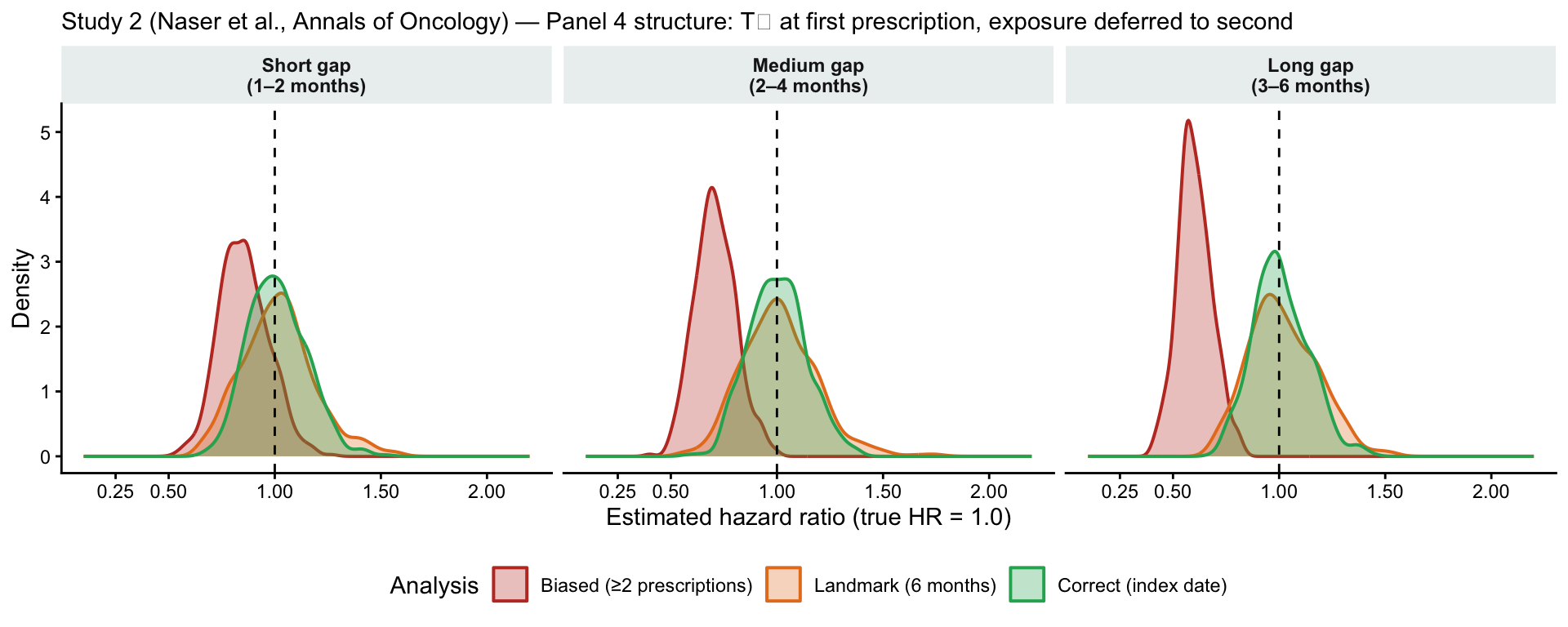
Parameters: 5,000 patients per replication, 500 replications. Cancer incidence calibrated to ~3% per year (a plausible composite rate for 13 obesity-associated cancers). Maximum follow-up 24 months, with administrative censoring uniformly distributed between 12 and 24 months, matching the reported IQR of 1–2 years. Three scenarios vary the Rx1→Rx2 gap (the immortal time duration): short (1–2 months), medium (2–4 months), long (3–6 months). Three analysis approaches are compared: the biased analysis (paper method: exposure classified only on ≥2 prescriptions), a landmark analysis at 6 months, and the correct analysis (exposure assigned at the first prescription, time zero).

library(survival)
library(ggplot2)
library(dplyr)
library(tidyr)

set.seed(2026)

n             <- 5000
n_sim         <- 500
lambda_cancer <- -log(0.97) / 12   # ~3% annual cancer incidence
max_fu        <- 24                 # 2-year maximum follow-up (months)

gap_scenarios <- list(
  "Short gap\n(1–2 months)"  = list(lo = 1, hi = 2),
  "Medium gap\n(2–4 months)" = list(lo = 2, hi = 4),
  "Long gap\n(3–6 months)"   = list(lo = 3, hi = 6)
)

cols <- c(
  "Biased (≥2 prescriptions)" = "#C0392B",
  "Landmark (6 months)"       = "#E67E22",
  "Correct (index date)"      = "#27AE60"
)

results_list <- lapply(seq_along(gap_scenarios), function(k) {
  sc   <- gap_scenarios[[k]]
  name <- names(gap_scenarios)[k]
  mat  <- matrix(NA_real_, nrow = n_sim, ncol = 3,
                 dimnames = list(NULL, c("biased", "landmark", "correct")))
  for (i in seq_len(n_sim)) {
    t_cancer <- rexp(n, rate = lambda_cancer)
    glp1     <- rep(c(TRUE, FALSE), each = n / 2)
    rx2_gap  <- ifelse(glp1, runif(n, sc$lo, sc$hi), NA_real_)
    t_cens   <- runif(n, max_fu * 0.5, max_fu)
    t_obs    <- pmin(t_cancer, t_cens)
    event    <- as.integer(t_cancer <= t_cens)

    # Biased: exposed only if survived cancer-free to Rx2
    exposed_b <- glp1 & (!event | t_cancer > rx2_gap)
    df_b <- data.frame(time = t_obs, event = event, exp = as.integer(exposed_b))
    mat[i, "biased"] <- tryCatch(
      exp(coef(coxph(Surv(time, event) ~ exp, data = df_b))),
      error = function(e) NA_real_)

    # Landmark at 6 months
    df_l <- df_b[df_b$time > 6, ]; df_l$time <- df_l$time - 6
    if (nrow(df_l) > 20)
      mat[i, "landmark"] <- tryCatch(
        exp(coef(coxph(Surv(time, event) ~ exp, data = df_l))),
        error = function(e) NA_real_)

    # Correct: exposure at time zero (first prescription)
    df_c <- data.frame(time = t_obs, event = event, exp = as.integer(glp1))
    mat[i, "correct"] <- tryCatch(
      exp(coef(coxph(Surv(time, event) ~ exp, data = df_c))),
      error = function(e) NA_real_)
  }
  as.data.frame(mat) %>% mutate(scenario = name)
})

all_res <- bind_rows(results_list) %>%
  pivot_longer(c(biased, landmark, correct), names_to = "analysis", values_to = "hr") %>%
  filter(!is.na(hr)) %>%
  mutate(
    analysis = factor(analysis,
      levels = c("biased", "landmark", "correct"),
      labels = c("Biased (≥2 prescriptions)", "Landmark (6 months)", "Correct (index date)")),
    scenario = factor(scenario, levels = names(gap_scenarios))
  )

# Summary table
all_res %>%
  group_by(scenario, analysis) %>%
  summarise(median_hr = round(median(hr), 2),
            p2_5      = round(quantile(hr, 0.025), 2),
            p97_5     = round(quantile(hr, 0.975), 2),
            .groups   = "drop") %>%
  knitr::kable(col.names = c("Rx1→Rx2 gap", "Analysis", "Median HR",
                              "2.5th percentile", "97.5th percentile"),
               caption = "Simulation results: true HR = 1.0 by construction. Reported overall HR in Naser et al.: 0.59.")

Simulation results: true HR = 1.0 by construction. Reported overall HR in Naser et al.: 0.59.

Rx1→Rx2 gap	Analysis	Median HR	2.5th percentile	97.5th percentile
Short gap
(1–2 months)	Biased (≥2 prescriptions)	0.85	0.65	1.10
Short gap
(1–2 months)	Landmark (6 months)	1.01	0.71	1.41
Short gap
(1–2 months)	Correct (index date)	1.00	0.77	1.29
Medium gap
(2–4 months)	Biased (≥2 prescriptions)	0.71	0.53	0.92
Medium gap
(2–4 months)	Landmark (6 months)	1.00	0.70	1.40
Medium gap
(2–4 months)	Correct (index date)	1.00	0.76	1.28
Long gap
(3–6 months)	Biased (≥2 prescriptions)	0.60	0.45	0.78
Long gap
(3–6 months)	Landmark (6 months)	1.00	0.73	1.34
Long gap
(3–6 months)	Correct (index date)	0.99	0.77	1.27

ggplot(all_res, aes(x = hr, fill = analysis, colour = analysis)) +
  geom_density(alpha = 0.30, linewidth = 0.7) +
  geom_vline(xintercept = 1.0, linetype = "dashed", colour = "black") +
  scale_fill_manual(values = cols) +
  scale_colour_manual(values = cols) +
  scale_x_continuous(limits = c(0.1, 2.2),
                     breaks = c(0.25, 0.5, 1.0, 1.5, 2.0)) +
  facet_wrap(~ scenario, ncol = 3) +
  labs(x = "Estimated hazard ratio (true HR = 1.0)", y = "Density",
       fill = "Analysis", colour = "Analysis",
       subtitle = "Study 2 (Naser et al., Annals of Oncology) — Panel 4 structure: T₀ at first prescription, exposure deferred to second") +
  theme_classic(base_size = 11) +
  theme(legend.position = "bottom",
        strip.background = element_rect(fill = "#ECF0F1", colour = NA),
        strip.text = element_text(face = "bold"))

Distribution of estimated hazard ratios across 500 Monte Carlo replications (true HR = 1.0). The long-gap scenario produces a median biased HR of 0.60, virtually identical to the reported overall HR of 0.59. The correct analysis centres on 1.0 in all scenarios.

The results are unambiguous. In the long-gap scenario (3–6 months of immortal time — fully plausible in a dataset where some patients delay refills), the biased analysis produces a median HR of 0.60, virtually identical to the paper’s reported overall HR of 0.59. The landmark analysis corrects the bias when its cut-point exceeds the maximum Rx2 gap, but this is not a general fix: for shorter immortal windows, or when the landmark is set before the Rx2 gap closes, bias persists. The correct analysis — assigning exposure at the first prescription — recovers the true HR of 1.0 in all scenarios.

The tirzepatide subgroup HR of 0.26 is not directly reproduced by this simulation, but the mechanism is clear from the scenario structure: tirzepatide users have shorter total follow-up (the drug was approved for obesity only in late 2023), meaning immortal time represents a larger fraction of their observation window. Shorter follow-up produces a lower biased HR — not a stronger drug effect.

Bottom line

This paper combines immortal time bias with reverse causation, a 2-year follow-up window that is biologically incoherent for cancer prevention, potential surveillance bias from differential healthcare contact, and a comparator-timing problem in the tirzepatide subgroup. The effect sizes are not just implausible — they are impossible given what we know about cancer biology and latency. The invocation of target trial emulation as a methodological strength, while failing to implement it correctly on the key dimension that matters, makes this more concerning rather than less. The authors and journal reviewers appear to have been persuaded by the framework’s name rather than its substance.

Where is the common sense (sniff test) of the reviewers and editors of a medical journal with an impact factor 65?

References

1.

Hernán MA, Wang W, Leaf DE. Target trial emulation: A framework for causal inference from observational data. JAMA [Internet]. 2022;328(24):2446–7. Available from: https://doi.org/10.1001/jama.2022.21383