Using an estimand‑driven Bayesian framework and the EXCEL aggregate trial data risk‑based quantities corresponding to clinically interpretable questions are estimated.
The EXCEL trial(Stone et al. 2019) randomized patients with left main coronary artery disease (LMCAD) to percutaneous coronary intervention (PCI) or coronary artery bypass grafting (CABG). A recent publication(Madhavan et al. 2026) from this dataset reported an increased 5-year risk of spontaneous myocardial infarction after PCI (adjusted hazard ratio [adjHR], 2.01; 95 CI, 1.29–3.15; P=0.002). It was also emphasized that although spontaneous MI (as a time-adjusted covariate) was a strong independent predictor of subsequent cardiovascular mortality (adjHR, 9.39; 95% CI, 5.22–16.87) this was independent of the initial revascularization choice (\(P_{interaction}\) = 0.23).
Analyses that condition on the occurrence of MI address post‑event prognosis but by ignoring differences in MI incidence provide an incomplete clinical answer regarding the safety of the initial revascularization choice. From a patient and clinician perspective, an approach focusing on an estimand that combines both incidence and prognosis jointly, complements conventional analyses of post‑MI hazard ratios.
Methods
Study Design and Data Sources
We performed an estimand‑driven Bayesian reanalysis of aggregate, arm‑level data reported from the EXCEL randomized trial comparing percutaneous coronary intervention (PCI) with coronary artery bypass grafting (CABG) in patients with left main coronary artery disease over 5 years of follow‑up.
Estimands
It is important to recognize that choosing an estimand, the specific quantity we aim to estimate and the clinical question it addresses, comes first and models, including survival models and hazard ratios are secondary tools, not absolute truths. The original analysis(Madhavan et al. 2026) emphasized the estimand of the mortality hazard ratio between the two initial revascualrization strategies conditional on a spontaneous MI having occurred. This manuscript emphasizes three prespecified, clinically interpretable estimands from a Bayesian perspective and evaluates each over the fixed 5‑year horizon:
Estimand #1. Incidence of spontaneous myocardial infarction according to original revascularization strategy
\(P(\text{MI} \mid \text{Treatment}=j)\)
Estimand #2. Post–myocardial infarction mortality according to original revascularization strategy
All estimands summarize observed risks under randomized treatment assignment and are descriptive. No causal mediation or mechanistic interpretation is implied. It is also worth noting that different estimands answer different clinical questions and no single number is “the” effect.
Statistical Analysis
Bayesian models were fit separately for MI incidence and post‑MI mortality, with all inference expressed on the probability scale. Posterior summaries include posterior means, 95% credible intervals (CrI), and posterior probabilities that risk under PCI exceeds that under CABG.
MI incidence was modeled using a binomial likelihood with a logit link. Mortality following spontaneous MI was modeled using a Gaussian likelihood as a normal approximation to a binomial model because only arm‑level estimates were available as expressed here
\[M_j \sim \text{Binomial}(N_j, p^{\text{MI}}_j)\] where \(N_j\) denote the number of patients receiving treatment \(j \in \{\text{PCI}, \text{CABG}\}\) and let \(M_j\) denotes the number experiencing a spontaneous MI during follow-up.
Posterior draws from these models were combined multiplicatively to obtain posterior distributions of the joint MI‑associated mortality estimand. Analyses were conducted in R using the brms, posterior, and ggplot2 packages. All statistical code is available online (https://github.com/brophyj/SpontaneousMI) and is fully reproducible.
Results
Incidence of Spontaneous Myocardial Infarction
The estimated 5‑year probabilities of spontaneous MI after PCI and CABG and the posterior median difference in spontaneous MI risk between strategies with their 95% credible intervals are reported in Table 1a. The posterior probability that \(P(\text{MI}\mid\text{PCI}) > P(\text{MI}\mid\text{CABG})\) was greater than 0.99.
Mortality After Spontaneous MI
The estimated mortality probabilities following spontaneous MI after PCI and CABG and the posterior median difference in mortality risks between strategies along with their 95% credible intervals are reported in Table 1b. The posterior probability that post‑MI mortality was higher following PCI was approximately 0.7.
Joint MI‑Associated Mortality Risk
When MI incidence and post‑MI mortality were considered jointly, the 5‑year probability of spontaneous MI followed by death was higher after PCI than CABG (Table 1c) at approximately 0.90.
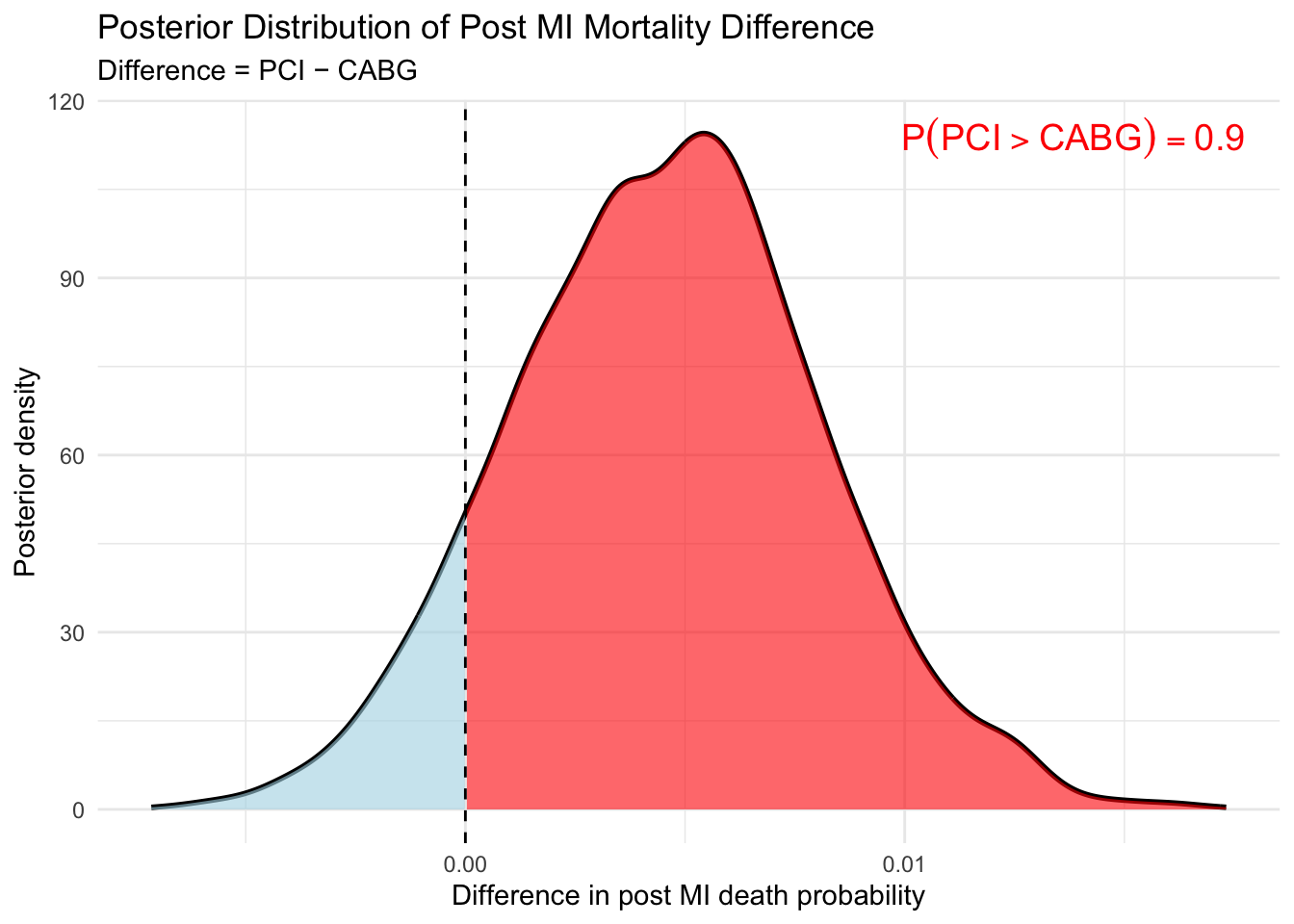
The posterior distribution of the absolute risk difference included small and near‑zero values (Figure), indicating uncertainty in magnitude despite consistent posterior support for direction.
Discussion
By focusing on explicitly defined, probability‑based estimands and expressing uncertainty directly on the risk scale, this analysis aims to complement, rather than replace, conventional time‑to‑event analyses and to reduce interpretive ambiguity arising from conditioning on post‑randomization events. This estimand‑driven Bayesian reanalysis demonstrates substantial posterior support that PCI is associated with a higher 5‑year burden of mortality following spontaneous myocardial infarction than CABG. Because each estimand is inherently probabilistic, a Bayesian framework provides a natural means of representing aand propagating uncertainty directly on the estimand scale through posterior distributions. This finding reflects both a clearly higher incidence of spontaneous MI after PCI and uncertainty‑weighted differences in post‑MI mortality. This joint estimand is descriptive rather than a formal causal mediation effect, as spontaneous MI is a post‑randomization event influenced by treatment. However, it provides a clinically meaningful summary of the overall risk of death following spontaneous MI under each revascularization strategy, and allows us to compute the posterior probability that PCI confers a higher MI‑associated mortality risk than CABG, jointly accounting for both event frequency and lethality.
Analyses conditioning on MI occurrence as in the original publication(Madhavan et al. 2026) target a restricted estimand — post‑event prognosis — and do not account for differences in MI frequency between revascularization strategies. In contrast, the joint estimand directly addresses a more clinically relevant question of overall disease burden as it captures both how often spontaneous MI occurs and how frequently it is followed by death according to the initial revascularization choice.
There are additional strengths to this analysis, illustrating how an estimand‑driven Bayesian framework can sharpen interpretation by aligning statistical inference directly with the clinical question being asked. By expressing uncertainty on the probability scale and by distinguishing clearly between event incidence, event severity, and their joint contribution to risk, the analysis highlights that differences in interpretation may arise from differences in estimands rather than disagreement about data or methodology.
There are also limitations to this analysis. First the estimands evaluated here are descriptive and do not imply causal mediation. Second, the absolute differences were modest and imprecisely estimated, and results are limited to the 5‑year follow‑up horizon. Finally, whether a posterior probability of this magnitude should influence clinical decision‑making depends on how clinicians and patients weigh modest absolute differences in MI associated mortality against other procedural risks, benefits, and patient‑specific considerations.
Conclusions
An estimand‑focused Bayesian reanalysis of the EXCEL trial indicates a high posterior probability that PCI confers a greater 5‑year burden of spontaneous MI‑associated mortality than CABG, although the absolute magnitude of difference remains uncertain. By following an estimand‑first workflow, the distinction between the clinical question, the estimand that encodes it, and the statistical model used for estimation, helps ensure that inference remains aligned with the intended interpretation.
Statistical code
Code
#---------------------------------------------# Model spontaneous MI incidence by treatment#---------------------------------------------dat_mi<-data.frame( arm =factor(c("CABG", "PCI")), # Treatment groups mi =c(29, 60), # Number of spontaneous MIs n =c(930, 952)# Number treated in each group)quiet_brms<-function(expr){invisible(capture.output(suppressMessages(expr)))}quiet_brms(fit_mi<-brm(mi|trials(n)~arm, # Binomial model for MI incidence data =dat_mi, family =binomial(link ="logit"), # Log link gives odds ratios (OR) prior =c(prior(normal(0, 1), class ="Intercept"), # Baseline MI riskprior(normal(0, 1), class ="b")# Log RR for PCI vs CABG), chains =4, iter =4000, refresh =0))post_mi<-as_draws_df(fit_mi)# -------------------------------------------------# Probability of spontaneous MI by treatment arm# (logit link → inverse-logit)# -------------------------------------------------p_mi_cabg<-plogis(post_mi$b_Intercept)p_mi_pci<-plogis(post_mi$b_Intercept+post_mi$b_armPCI)ci_cabg<-quantile(p_mi_cabg, c(0.025, 0.975))ci_pci<-quantile(p_mi_pci, c(0.025, 0.975))diff_mi<-p_mi_pci-p_mi_cabgci_diff_mi<-quantile(diff_mi, c(0.025, 0.975))
Code
#----------------------------------------------------# Model mortality risk conditional on spontaneous MI#----------------------------------------------------dat_death<-data.frame( arm =factor(c("CABG", "PCI")), yi =c(8.22, 11.73), # Death risk (%) after MI sei =c(5.83, 4.56)# Standard error of risk estimate)quiet_brms(fit_death<-brm(yi|se(sei)~arm, # Normal approximation to binomial data =dat_death, family =gaussian(), prior =prior(normal(0, 10), class ="Intercept"), chains =4, iter =4000, refresh =0))post_d<-as_draws_df(fit_death)# -------------------------------------------------# Probability of death conditional on spontaneous MI# (entered as percentages → convert to probabilities)# -------------------------------------------------p_d_cabg<-post_d$b_Intercept/100p_d_pci<-(post_d$b_Intercept+post_d$b_armPCI)/100ci_p_d_cabg<-quantile(p_d_cabg, c(0.025, 0.975))ci_p_d_pci<-quantile(p_d_pci, c(0.025, 0.975))diff_death<-p_d_pci-p_d_cabgci_diff_death<-quantile(diff_death, c(0.025, 0.975))diff_death_prob<-mean(diff_death>0)
Code
# Align posterior drawsn_draw<-min(nrow(post_mi), nrow(post_d))post_mi<-post_mi[1:n_draw, ]post_d<-post_d[1:n_draw, ]# -------------------------------------------------# Probability of spontaneous MI by treatment arm# (logit link → inverse-logit)# -------------------------------------------------p_mi_cabg<-plogis(post_mi$b_Intercept)p_mi_pci<-plogis(post_mi$b_Intercept+post_mi$b_armPCI)# -------------------------------------------------# Probability of death conditional on spontaneous MI# (entered as percentages → convert to probabilities)# no need for plogis since gaussian model is already on probability scale# -------------------------------------------------p_d_cabg<-post_d$b_Intercept/100p_d_pci<-(post_d$b_Intercept+post_d$b_armPCI)/100# -------------------------------------------------# Truncate probabilities to [0,1] due to linear model simpler than alternative# Replace gaussian with logit‑normal likelihood # brm(yi | se(sei) ~ arm,family = gaussian(link = "logit"))# Then need to apply inverse logit# -------------------------------------------------p_d_cabg<-pmin(pmax(p_d_cabg, 0), 1)p_d_pci<-pmin(pmax(p_d_pci, 0), 1)# -------------------------------------------------# Overall risk of death MI‑associated mortality risk# -------------------------------------------------risk_cabg<-p_mi_cabg*p_d_cabgrisk_pci<-p_mi_pci*p_d_pcici_risk_cabg<-quantile(risk_cabg, c(0.025, .50, 0.975))ci_risk_pci<-quantile(risk_pci, c(0.025, .50, 0.975))diff_overall<-risk_pci-risk_cabgp_combined<-mean(diff_overall>0)ci_diff_overall<-quantile(diff_overall, c(0.025, 0.5, 0.975))
Posterior plot for the combined two‑model estimand
Code
library(ggplot2)# Posterior probability (define explicitly)p_combined<-mean(diff_overall>0)plot_df<-data.frame(diff =diff_overall)# Compute ONE normalized density via ggplotdensity_data<-ggplot_build(ggplot(plot_df, aes(x =diff))+geom_density())$data[[1]]ggplot()+# Full posterior densitygeom_line( data =density_data,aes(x =x, y =density), linewidth =1)+# Area where diff <= 0geom_area( data =subset(density_data, x<=0),aes(x =x, y =density), fill ="lightblue", alpha =0.6)+# Area where diff > 0 (AUC = posterior probability)geom_area( data =subset(density_data, x>0),aes(x =x, y =density), fill ="red", alpha =0.6)+geom_vline(xintercept =0, linetype ="dashed")+annotate("text", x =Inf, y =Inf, label =sprintf("P(PCI > CABG) == %.2f", p_combined), parse =TRUE, hjust =1.1, vjust =1.4, color ="red", size =5)+labs( title ="Posterior Distribution of Post MI Mortality Difference", subtitle ="Difference = PCI − CABG", x ="Difference in post MI death probability", y ="Posterior density")+theme_minimal()
The posterior density of the difference in MI‑associated mortality risk \[
\Delta =
P(\text{MI}\mid\text{PCI})P(\text{Death}\mid\text{MI},\text{PCI})
-
P(\text{MI}\mid\text{CABG})P(\text{Death}\mid\text{MI},\text{CABG})
\] is shown above.
The shaded red region corresponds to posterior draws where \(\Delta > 0\). The total area of this region equals \[
P(\Delta > 0 \mid \text{data}) \approx 0.90,
\] representing the posterior probability that PCI confers a higher overall risk of death following spontaneous myocardial infarction.
Tables
Table 1a
Incidence of Spontaneous Myocardial Infarction
Posterior summaries over 5‑year follow‑up
Strategy
5-year MI risk (%)
Risk difference (per 1,000)
CABG
3.3 (2.3–4.5)
—
PCI
6.4 (4.9–8.0)
—
PCI − CABG
—
30.5 (11.5–49.8)
Values are posterior means with 95% credible intervals.
Posterior probability MI risk is higher after PCI: 1.00
Table 1b
Mortality Following Spontaneous Myocardial Infarction
Posterior summaries conditional on MI occurrence
Strategy
Post-MI mortality (%)
Risk difference (per 1,000)
CABG
7.0 (-4.4–17.7)
—
PCI
10.8 (2.2–19.4)
—
PCI − CABG
—
41.2 (-100.7–187.2)
Values are posterior means with 95% credible intervals.
Posterior probability post‑MI mortality is higher after PCI: 0.72
Table 1c
Joint 5‑year Probability of Spontaneous MI and Subsequent Death
Descriptive joint estimand
Quantity
Estimate
Joint MI–death risk after CABG (per 1,000)
2.2 (0.0–6.2)
Joint MI–death risk after PCI (per 1,000)
6.8 (1.4–13.0)
Absolute difference in joint MI–death risk (PCI − CABG, per 1,000)
4.6 (-2.2–11.7)
Posterior probability joint risk is higher after PCI
0.90
References
Madhavan, M. V., J. Gregson, B. Redfors, S. Chen, 3rd Sabik J. F., A. Fujino, L. N. Kotinkaduwa, et al. 2026. “Spontaneous Myocardial Infarction After Left Main Revascularization: The EXCEL Trial.” Journal Article. Circulation 153 (12): 890–901. https://doi.org/10.1161/CIRCULATIONAHA.125.075875.
Stone, G. W., A. P. Kappetein, J. F. Sabik, S. J. Pocock, M. C. Morice, J. Puskas, D. E. Kandzari, et al. 2019. “Five-Year Outcomes After PCI or CABG for Left Main Coronary Disease.” Journal Article. N Engl J Med 381 (19): 1820–30. https://doi.org/10.1056/NEJMoa1909406.
---title: "Spontaneous Myocardial Infarction After Left Main Revascularization"subtitle: "An Estimand Focused Reanalysis" description: "Using an estimand‑driven Bayesian framework and the EXCEL aggregate trial data risk‑based quantities corresponding to clinically interpretable questions are estimated."author: - name: Jay Brophy url: https://brophyj.github.io/ orcid: 0000-0001-8049-6875 affiliation: McGill University Dept Medicine, Epidemiology & Biostatistics affiliation-url: https://mcgill.cacategories: [RCT, Bayesian]image: preview-image.jpgcitation: url: https://brophyj.com/posts/2026-04-21-my-blog-post/ date: 2026-04-20T14:39:55-05:00lastmod: 2026-04-20T14:39:55-05:00featured: truedraft: false# Focal points: Smart, Center, TopLeft, Top, TopRight, Left, Right, BottomLeft, Bottom, BottomRight.projects: []format: html: code-fold: true code-tools: true # optional: adds copy/download buttons keep_md: true self_contained: trueeditor_options: markdown: wrap: sentencebiblio-style: apalikebibliography: references.bib---```{r}#| label: setup#| include: falsesuppressPackageStartupMessages({library(tidyverse)library(brms)library(posterior)})set.seed(20251109)knitr::opts_chunk$set(fig.align ="center")theme_set(theme_minimal(base_size =13) +theme(panel.grid.minor =element_blank(),plot.title =element_text(face ="bold"),plot.subtitle =element_text(color ="grey40") ))```## BackgroundThe EXCEL trial[@excel] randomized patients with left main coronary artery disease (LMCAD) to percutaneous coronary intervention (PCI) or coronary artery bypass grafting (CABG). A recent publication[@spontaneousMI] from this dataset reported an increased 5-year risk of spontaneous myocardial infarction after PCI (adjusted hazard ratio [adjHR], 2.01; 95 CI, 1.29–3.15; P=0.002). It was also emphasized that although spontaneous MI (as a time-adjusted covariate) was a strong independent predictor of subsequent cardiovascular mortality (adjHR, 9.39; 95% CI, 5.22–16.87) this was independent of the initial revascularization choice ($P_{interaction}$ = 0.23). Analyses that condition on the occurrence of MI address post‑event prognosis but by ignoring differences in MI incidence provide an incomplete clinical answer regarding the safety of the initial revascularization choice. From a patient and clinician perspective, an approach focusing on an estimand that combines both incidence and prognosis jointly, complements conventional analyses of post‑MI hazard ratios. ## Methods### Study Design and Data SourcesWe performed an estimand‑driven Bayesian reanalysis of aggregate, arm‑level data reported from the EXCEL randomized trial comparing percutaneous coronary intervention (PCI) with coronary artery bypass grafting (CABG) in patients with left main coronary artery disease over 5 years of follow‑up.### EstimandsIt is important to recognize that choosing an estimand, the specific quantity we aim to estimate and the clinical question it addresses, comes first and models, including survival models and hazard ratios are secondary tools, not absolute truths. The original analysis[@spontaneousMI] emphasized the estimand of the mortality hazard ratio between the two initial revascualrization strategies conditional on a spontaneous MI having occurred. This manuscript emphasizes three prespecified, clinically interpretable estimands from a Bayesian perspective and evaluates each over the fixed 5‑year horizon:**Estimand #1. Incidence of spontaneous myocardial infarction according to original revascularization strategy**$P(\text{MI} \mid \text{Treatment}=j)$**Estimand #2. Post–myocardial infarction mortality according to original revascularization strategy**$P(\text{Death} \mid \text{MI}, \text{Treatment}=j)$.**Estimand #3.** Joint MI‑associated mortality burden: $P(\text{MI} \mid j)\times P(\text{Death} \mid \text{MI}, j)$.All estimands summarize observed risks under randomized treatment assignment and are descriptive. No causal mediation or mechanistic interpretation is implied. It is also worth noting that different estimands answer different clinical questions and no single number is “the” effect.### Statistical AnalysisBayesian models were fit separately for MI incidence and post‑MI mortality, with all inference expressed on the probability scale. Posterior summaries include posterior means, 95% credible intervals (CrI), and posterior probabilities that risk under PCI exceeds that under CABG.MI incidence was modeled using a binomial likelihood with a logit link. Mortality following spontaneous MI was modeled using a Gaussian likelihood as a normal approximation to a binomial model because only arm‑level estimates were available as expressed here $$M_j \sim \text{Binomial}(N_j, p^{\text{MI}}_j)$$where $N_j$ denote the number of patients receiving treatment $j \in \{\text{PCI}, \text{CABG}\}$ and let $M_j$ denotes the number experiencing a spontaneous MI during follow-up. Posterior draws from these models were combined multiplicatively to obtain posterior distributions of the joint MI‑associated mortality estimand.Analyses were conducted in R using the `brms`, `posterior`, and `ggplot2` packages. All statistical code is available online (https://github.com/brophyj/SpontaneousMI) and is fully reproducible.## Results### Incidence of Spontaneous Myocardial Infarction The estimated 5‑year probabilities of spontaneous MI after PCI and CABG and the posterior median difference in spontaneous MI risk between strategies with their 95% credible intervals are reported in Table 1a. The posterior probability that $P(\text{MI}\mid\text{PCI}) > P(\text{MI}\mid\text{CABG})$ was greater than 0.99.### Mortality After Spontaneous MIThe estimated mortality probabilities following spontaneous MI after PCI and CABG and the posterior median difference in mortality risks between strategies along with their 95% credible intervals are reported in Table 1b. The posterior probability that post‑MI mortality was higher following PCI was approximately 0.7. ### Joint MI‑Associated Mortality RiskWhen MI incidence and post‑MI mortality were considered jointly, the 5‑year probability of spontaneous MI followed by death was higher after PCI than CABG (Table 1c) at approximately 0.90.The posterior distribution of the absolute risk difference included small and near‑zero values (Figure), indicating uncertainty in magnitude despite consistent posterior support for direction.## DiscussionBy focusing on explicitly defined, probability‑based estimands and expressing uncertainty directly on the risk scale, this analysis aims to complement, rather than replace, conventional time‑to‑event analyses and to reduce interpretive ambiguity arising from conditioning on post‑randomization events. This estimand‑driven Bayesian reanalysis demonstrates substantial posterior support that PCI is associated with a higher 5‑year burden of mortality following spontaneous myocardial infarction than CABG. Because each estimand is inherently probabilistic, a Bayesian framework provides a natural means of representing aand propagating uncertainty directly on the estimand scale through posterior distributions. This finding reflects both a clearly higher incidence of spontaneous MI after PCI and uncertainty‑weighted differences in post‑MI mortality. This joint estimand is descriptive rather than a formal causal mediation effect, as spontaneous MI is a post‑randomization event influenced by treatment. However, it provides a clinically meaningful summary of the overall risk of death following spontaneous MI under each revascularization strategy, and allows us to compute the posterior probability that PCI confers a higher MI‑associated mortality risk than CABG, jointly accounting for both event frequency and lethality. Analyses conditioning on MI occurrence as in the original publication[@spontaneousMI] target a restricted estimand — post‑event prognosis — and do not account for differences in MI frequency between revascularization strategies. In contrast, the joint estimand directly addresses a more clinically relevant question of overall disease burden as it captures both how often spontaneous MI occurs and how frequently it is followed by death according to the initial revascularization choice. There are additional strengths to this analysis, illustrating how an estimand‑driven Bayesian framework can sharpen interpretation by aligning statistical inference directly with the clinical question being asked. By expressing uncertainty on the probability scale and by distinguishing clearly between event incidence, event severity, and their joint contribution to risk, the analysis highlights that differences in interpretation may arise from differences in estimands rather than disagreement about data or methodology. There are also limitations to this analysis. First the estimands evaluated here are descriptive and do not imply causal mediation. Second, the absolute differences were modest and imprecisely estimated, and results are limited to the 5‑year follow‑up horizon. Finally, whether a posterior probability of this magnitude should influence clinical decision‑making depends on how clinicians and patients weigh modest absolute differences in MI associated mortality against other procedural risks, benefits, and patient‑specific considerations. ## ConclusionsAn estimand‑focused Bayesian reanalysis of the EXCEL trial indicates a high posterior probability that PCI confers a greater 5‑year burden of spontaneous MI‑associated mortality than CABG, although the absolute magnitude of difference remains uncertain. By following an estimand‑first workflow, the distinction between the clinical question, the estimand that encodes it, and the statistical model used for estimation, helps ensure that inference remains aligned with the intended interpretation. ### Statistical code```{r cache=TRUE}#---------------------------------------------# Model spontaneous MI incidence by treatment#---------------------------------------------dat_mi <-data.frame(arm =factor(c("CABG", "PCI")), # Treatment groupsmi =c(29, 60), # Number of spontaneous MIsn =c(930, 952) # Number treated in each group)quiet_brms <-function(expr) {invisible(capture.output(suppressMessages(expr) ))}quiet_brms(fit_mi <-brm( mi |trials(n) ~ arm, # Binomial model for MI incidencedata = dat_mi,family =binomial(link ="logit"), # Log link gives odds ratios (OR)prior =c(prior(normal(0, 1), class ="Intercept"), # Baseline MI riskprior(normal(0, 1), class ="b") # Log RR for PCI vs CABG ),chains =4, iter =4000, refresh =0))post_mi <-as_draws_df(fit_mi)# -------------------------------------------------# Probability of spontaneous MI by treatment arm# (logit link → inverse-logit)# -------------------------------------------------p_mi_cabg <-plogis(post_mi$b_Intercept)p_mi_pci <-plogis(post_mi$b_Intercept + post_mi$b_armPCI)ci_cabg <-quantile(p_mi_cabg, c(0.025, 0.975))ci_pci <-quantile(p_mi_pci, c(0.025, 0.975))diff_mi <- p_mi_pci - p_mi_cabgci_diff_mi <-quantile(diff_mi, c(0.025, 0.975))``````{r print1, echo=FALSE, message=FALSE, warning=FALSE, eval=FALSE}# eval=FALSE for submission as output printed in Tablescat(sprintf("Estimated probability of spontaneous MI after CABG: %.1f%% (95%% credible interval %.1f%% to %.1f%%)\n",mean(p_mi_cabg) *100, ci_cabg[1] *100, ci_cabg[2] *100 ))cat(sprintf("Estimated probability of spontaneous MI after PCI: %.1f%% (95%% credible interval %.1f%% to %.1f%%)\n",mean(p_mi_pci) *100, ci_pci[1] *100, ci_pci[2] *100 ))cat(sprintf("The posterior median difference in spontaneous MI risk is %.1f excess MIs per 1,000 patients treated with PCI vs CABG (95%% credible interval %.1f to %.1f per 1,000).",mean(diff_mi) *1000, ci_diff_mi[1] *1000, ci_diff_mi[2] *1000 ))``````{r cache=TRUE}#----------------------------------------------------# Model mortality risk conditional on spontaneous MI#----------------------------------------------------dat_death <-data.frame(arm =factor(c("CABG", "PCI")),yi =c(8.22, 11.73), # Death risk (%) after MIsei =c(5.83, 4.56) # Standard error of risk estimate)quiet_brms(fit_death <-brm( yi |se(sei) ~ arm, # Normal approximation to binomialdata = dat_death,family =gaussian(),prior =prior(normal(0, 10), class ="Intercept"),chains =4, iter =4000, refresh =0))post_d <-as_draws_df(fit_death)# -------------------------------------------------# Probability of death conditional on spontaneous MI# (entered as percentages → convert to probabilities)# -------------------------------------------------p_d_cabg <- post_d$b_Intercept /100p_d_pci <- (post_d$b_Intercept + post_d$b_armPCI) /100ci_p_d_cabg <-quantile(p_d_cabg, c(0.025, 0.975))ci_p_d_pci <-quantile(p_d_pci, c(0.025, 0.975))diff_death <- p_d_pci - p_d_cabgci_diff_death <-quantile(diff_death, c(0.025, 0.975))diff_death_prob <-mean(diff_death >0)``````{r print2, echo=FALSE, message=FALSE, warning=FALSE, eval=FALSE}# eval=FALSE for submission as output printed in Tablescat(sprintf("Estimated probability of death after spontaneous MI in PCI patients: %.1f%% (95%% credible interval %.1f%% to %.1f%%)\n",mean(p_d_pci) *100, ci_p_d_pci[1] *100, ci_p_d_pci[2] *100 ))cat(sprintf("Estimated probability of death after spontaneous MI in CABG patients: %.1f%% (95%% credible interval %.1f%% to %.1f%%)\n",mean(p_d_cabg) *100, ci_p_d_cabg[1] *100, ci_p_d_cabg[2] *100 ))cat(sprintf("The posterior median difference in post-MI mortality risk is %.1f excess deaths per 1,000 patients treated with PCI vs CABG (95%% credible interval %.1f to %.1f per 1,000).",mean(diff_death) *1000 , ci_diff_death[1] *1000, ci_diff_death[2] *1000 ))cat(sprintf("Posterior probability that post-MI mortality risk is higher after PCI than CABG: %.0f %%", diff_death_prob*100 ))``````{r}# Align posterior drawsn_draw <-min(nrow(post_mi), nrow(post_d))post_mi <- post_mi[1:n_draw, ]post_d <- post_d[1:n_draw, ]# -------------------------------------------------# Probability of spontaneous MI by treatment arm# (logit link → inverse-logit)# -------------------------------------------------p_mi_cabg <-plogis(post_mi$b_Intercept)p_mi_pci <-plogis(post_mi$b_Intercept + post_mi$b_armPCI)# -------------------------------------------------# Probability of death conditional on spontaneous MI# (entered as percentages → convert to probabilities)# no need for plogis since gaussian model is already on probability scale# -------------------------------------------------p_d_cabg <- post_d$b_Intercept /100p_d_pci <- (post_d$b_Intercept + post_d$b_armPCI) /100# -------------------------------------------------# Truncate probabilities to [0,1] due to linear model simpler than alternative# Replace gaussian with logit‑normal likelihood # brm(yi | se(sei) ~ arm,family = gaussian(link = "logit"))# Then need to apply inverse logit# -------------------------------------------------p_d_cabg <-pmin(pmax(p_d_cabg, 0), 1)p_d_pci <-pmin(pmax(p_d_pci, 0), 1)# -------------------------------------------------# Overall risk of death MI‑associated mortality risk# -------------------------------------------------risk_cabg <- p_mi_cabg * p_d_cabgrisk_pci <- p_mi_pci * p_d_pcici_risk_cabg <-quantile(risk_cabg, c(0.025, .50, 0.975))ci_risk_pci <-quantile(risk_pci, c(0.025, .50, 0.975))diff_overall <- risk_pci - risk_cabgp_combined <-mean(diff_overall >0)ci_diff_overall <-quantile(diff_overall, c(0.025, 0.5, 0.975))``````{r print3, echo=FALSE, message=FALSE, warning=FALSE, eval=FALSE}# eval=FALSE for submission as output printed in Tablescat(sprintf("Following a spontaneous MI, PCI has a %.2f posterior probability of a higher death risk than CABG:", p_combined ))cat(sprintf("The posterior median difference in post spontaneous MI mortality risk is %.1f excess deaths per 1,000 patients between those treated initially with PCI vs CABG (95%% credible interval %.1f to %.1f per 1,000).", ci_diff_overall[2] *1000, ci_diff_overall[1] *1000, ci_diff_overall[3] *1000 ))```### Posterior plot for the combined two‑model estimand```{r}library(ggplot2)# Posterior probability (define explicitly)p_combined <-mean(diff_overall >0)plot_df <-data.frame(diff = diff_overall)# Compute ONE normalized density via ggplotdensity_data <-ggplot_build( ggplot(plot_df, aes(x = diff)) +geom_density())$data[[1]]ggplot() +# Full posterior densitygeom_line(data = density_data,aes(x = x, y = density),linewidth =1 ) +# Area where diff <= 0geom_area(data =subset(density_data, x <=0),aes(x = x, y = density),fill ="lightblue",alpha =0.6 ) +# Area where diff > 0 (AUC = posterior probability)geom_area(data =subset(density_data, x >0),aes(x = x, y = density),fill ="red",alpha =0.6 ) +geom_vline(xintercept =0, linetype ="dashed") +annotate("text",x =Inf, y =Inf,label =sprintf("P(PCI > CABG) == %.2f", p_combined),parse =TRUE,hjust =1.1,vjust =1.4,color ="red",size =5) +labs(title ="Posterior Distribution of Post MI Mortality Difference",subtitle ="Difference = PCI − CABG",x ="Difference in post MI death probability",y ="Posterior density" ) +theme_minimal()```The posterior density of the difference in MI‑associated mortality risk$$\Delta =P(\text{MI}\mid\text{PCI})P(\text{Death}\mid\text{MI},\text{PCI})-P(\text{MI}\mid\text{CABG})P(\text{Death}\mid\text{MI},\text{CABG})$$is shown above.The shaded red region corresponds to posterior draws where $\Delta > 0$.The total area of this region equals$$P(\Delta > 0 \mid \text{data}) \approx 0.90,$$representing the posterior probability that PCI confers a higher overallrisk of death following spontaneous myocardial infarction.### Tables**Table 1a**```{r table1, echo=FALSE, message=FALSE, warning=FALSE}library(dplyr)mi_cabg_mean <-mean(p_mi_cabg) *100mi_cabg_ci <- ci_cabg *100mi_pci_mean <-mean(p_mi_pci) *100mi_pci_ci <- ci_pci *100mi_diff_mean <-mean(diff_mi) *1000mi_diff_ci <- ci_diff_mi *1000fmt_pct <-function(m, ci) sprintf("%.1f (%.1f–%.1f)", m, ci[1], ci[2])fmt_diff <-function(m, ci) sprintf("%.1f (%.1f–%.1f)", m, ci[1], ci[2])table_mi_incidence <-tibble(Strategy =c("CABG", "PCI", "PCI − CABG"),`5-year MI risk (%)`=c(fmt_pct(mi_cabg_mean, mi_cabg_ci),fmt_pct(mi_pci_mean, mi_pci_ci),"—" ),`Risk difference (per 1,000)`=c("—", "—", fmt_diff(mi_diff_mean, mi_diff_ci) ))if (knitr::opts_knit$get("rmarkdown.pandoc.to") =="docx") {cat("**Table 1a. Incidence of Spontaneous Myocardial Infarction**\n\n")suppressPackageStartupMessages(library(flextable))flextable(table_mi_incidence) |>align(align ="center", part ="all") |>bold(part ="header") |>autofit() |>add_footer_lines(values =c("Values are posterior means with 95% credible intervals.",sprintf("Posterior probability MI risk is higher after PCI: %.2f",mean(diff_mi >0) ) ) )} else {suppressPackageStartupMessages(library(gt))gt(table_mi_incidence) |>tab_header(title ="Incidence of Spontaneous Myocardial Infarction",subtitle ="Posterior summaries over 5‑year follow‑up" ) |>cols_align("center", everything()) |>tab_source_note("Values are posterior means with 95% credible intervals.") |>tab_source_note(sprintf("Posterior probability MI risk is higher after PCI: %.2f",mean(diff_mi >0) ))}```**Table 1b**```{r table2, echo=FALSE, message=FALSE, warning=FALSE}library(dplyr)death_cabg_mean <-mean(p_d_cabg) *100death_cabg_ci <- ci_p_d_cabg *100death_pci_mean <-mean(p_d_pci) *100death_pci_ci <- ci_p_d_pci *100death_diff_mean <-mean(diff_death) *1000death_diff_ci <- ci_diff_death *1000table_post_mi <-tibble(Strategy =c("CABG", "PCI", "PCI − CABG"),`Post-MI mortality (%)`=c(fmt_pct(death_cabg_mean, death_cabg_ci),fmt_pct(death_pci_mean, death_pci_ci),"—" ),`Risk difference (per 1,000)`=c("—", "—", fmt_diff(death_diff_mean, death_diff_ci) ))if (knitr::opts_knit$get("rmarkdown.pandoc.to") =="docx") {cat("**Table 1b. Mortality Following Spontaneous Myocardial Infarction**\n\n")suppressPackageStartupMessages(library(flextable))flextable(table_post_mi) |>align(align ="center", part ="all") |>bold(part ="header") |>autofit() |>add_footer_lines(values =c("Values are posterior means with 95% credible intervals.",sprintf("Posterior probability post‑MI mortality is higher after PCI: %.2f",mean(diff_death >0) ) ) )} else {suppressPackageStartupMessages(library(gt))gt(table_post_mi) |>tab_header(title ="Mortality Following Spontaneous Myocardial Infarction",subtitle ="Posterior summaries conditional on MI occurrence" ) |>cols_align("center", everything()) |>tab_source_note("Values are posterior means with 95% credible intervals.") |>tab_source_note(sprintf("Posterior probability post‑MI mortality is higher after PCI: %.2f",mean(diff_death >0) ))}```**Table 1c**```{r table3, echo=FALSE, message=FALSE, warning=FALSE}joint_cabg <- ci_risk_cabg *1000joint_pci <- ci_risk_pci *1000joint_diff <- ci_diff_overall *1000table_joint <-tibble(Quantity =c("Joint MI–death risk after CABG (per 1,000)","Joint MI–death risk after PCI (per 1,000)","Absolute difference in joint MI–death risk (PCI − CABG, per 1,000)","Posterior probability joint risk is higher after PCI" ),Estimate =c(sprintf("%.1f (%.1f–%.1f)", joint_cabg[2], joint_cabg[1], joint_cabg[3]),sprintf("%.1f (%.1f–%.1f)", joint_pci[2], joint_pci[1], joint_pci[3]),sprintf("%.1f (%.1f–%.1f)", joint_diff[2], joint_diff[1], joint_diff[3]),sprintf("%.2f", p_combined) ))if (knitr::opts_knit$get("rmarkdown.pandoc.to") =="docx") {cat("**Table 1c. Joint 5‑year Probability of Spontaneous MI and Subsequent Death (MI‑associated mortality)**\n\n")suppressPackageStartupMessages(library(flextable))flextable(table_joint) |>align(j =1, align ="left", part ="body") |>align(j =2, align ="center", part ="body") |>bold(part ="header") |>autofit() |>add_footer_lines("Joint risk is defined as P(MI) × P(Death | MI), evaluated separately by treatment arm." )} else {suppressPackageStartupMessages(library(gt))gt(table_joint) |>tab_header(title ="Joint 5‑year Probability of Spontaneous MI and Subsequent Death",subtitle ="Descriptive joint estimand" ) |>cols_align("left", 1) |>cols_align("center", 2)}```## References